 is a function from
  to
to  . Then we can define a
sequence
  as follows.
Suppose  is a function from
  to
to  . Then we can define a
sequence
  as follows.

where a is some fixed number we choose. In class we talked about sequences generated this way and gave some examples of how such sequences might arise in models of population growth. For convenience, we will call a sequence generated in this way a recursive sequence.
Studying sequences generated in this way has also been of great interest in the area of mathematics called Dynamical Systems. In fact it was in such systems that the phenomenon of deterministic chaos was first understood. In this project you will investigate the convergence of sequences generated in this way.
To help you out, some simple Maple procedures have been written as
part of the CalcP package. These
programs will be useful in generating and plotting recursive sequences
and are described in a section at the end of this handout. A brief
description of each command also appears below. Each of these
procedures requires you to define a value for the variable start
and a procedure func before you read them in. The value of the
variable start is used for  and the procedure func is
used to generate the sequence. To read these procedures in, use the
read command exactly as in the examples. Note that in the
read command, the filename must be enclosed in backquotes,(`).
 . The syntax is
 Recur(f,start,n);, where f is a function
or expression, start is the value of  , and n is an integer.
Sequence(f,start,n);,
where the arguments have the same meaning as for Recur.
PlotSeq(f,start,);,
where the arguments have the same meaning as for Recur.
 and y=x. The syntax is
ShowSeq(f,start,n);. As usual, the arguments have the same
meaning as for Recur.
The main question in working with a recursive sequence is to determine
the behavior of the sequence for large values of n. If the sequence
converges, then the interpretation is straightforward. It turns out,
however, that there are several ways in which the sequence can
diverge. One way is for the sequence to be asymptotically
periodic, which we define as follows. We say that a sequence is
periodic with period K if  for sufficiently large n
and K is the smallest integer for which this is true. For example,
every constant sequence is 1-periodic, while the sequence
 is periodic with period 2. A sequence is
asymptotically of period K if it approaches a K-periodic
sequence. The sequence
  , for example, is
asymptotically of period 2. Sequences which are bounded but not
asymptotically periodic are called chaotic.
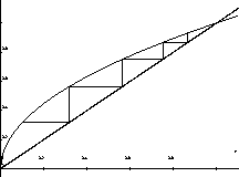
There is a very useful graphical procedure for plotting recursive
sequences. Given a value for  , the value of
  can be obtained
by finding
  . If we draw a horizontal line from the point
 to the line y=x we arrive at the point
  . A
vertical line from this point intersects the graph of
  at the
point
  , whose y coordinate is the next term in the
sequence. This procedure can be continued as long as you wish. An
example of the first five steps of this algorithm for
  and
and  is shown in Figure 2 at the end of this
handout.
The goal of this project is for you to discover criteria that will let you predict convergence or divergence of recursive sequences. In this section you are led through a series of exercises that will provide you with the answers you need.
 and
and  .
.
 and a=2.
 and
and  .
.
 and
and  .
.
 and
and  .
.
 and
and  .
.
 . Solutions of the equation
  are called fixed
points of the function f.
 if f is a continuous function.
 such that the sequence converges to L?
 , where
m is a parameter,
  . Every function in this family has a
single fixed point at x=1. Find the values of m for which
recursive sequences converge to this fixed point. (It turns out that
convergence or divergence is independent of the starting value you
choose, so you don't need to worry about this.)
The following result may be useful to you.
If there is a number r and a constant c with 0 <c <1 such that

then the sequence  converges to r.
 is continuously differentiable and L satisfies
 . Based on your answer to the previous part, make a conjecture
on f that will guarantee that a recursive sequence that has
  close to L will converge to L. Try to prove your conjecture.
Your project report should be about convergence of recursive sequences to fixed points of functions. It should not be just a description of what you did in the exercises. Write your report as if you were explaining what you discovered to a friend. The examples in the exercises are just examples; they can be used to motivate your results but they are not the primary results. Use the same structure for your report that you used for the first project.
These procedures will help you in generating and plotting recursive
sequences. Each of these procedures requires you to define a value for
the variable start and a procedure func before you read
them in. The value of the variable start is used for  and
the procedure func is used to generate the sequence. To read
these procedures in, use the read command exactly as in the
examples. Note that in the read command, the filename must be
enclosed in backquotes,(`). If you want to see what these procedures
look like, you can copy the files to your home directory. If you are
not sure how to do this, ask me, one of the lab monitors, or a friend
who knows UNIX.
 for a recursive sequence. The syntax for this procedure is
Recur(f,start,n), where f is a function
or expression, start is the value of  , and n is an
integer. The following sample Maple session shows how to load the
CalcP package
and use this procedure with the function
  .
.
> with(CalcP);

> f := x -> sqrt(x);

> Recur(f,0.1,1);

> Recur(f,0.1,2);

> Recur(f,0.1,10);

Sequence(f,start,n);, will print out the values  of the recursive sequence. The following example shows how to
use this procedure. Note that the CalcP package only needs to be
loaded once, so you don't have to use the with(CalcP); command again.
> Sequence(f,0.1,4);

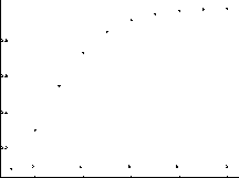
 for i from 1 to n. The following example produced the
plot in Figure 1.
> PlotSeq(f,0.1,10);
> ShowSeq(f,0.1,5);

Figure: First ten iterates for the function  with
with  .
.

Figure: Graphical algorithm for the first five iterates of  with
with  .
.