


Next: About this document ...
Up: lab_template
Previous: lab_template
Subsections
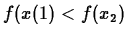
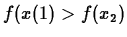
Suppose that  is a differentiable function. Then we
know that the value of
is a differentiable function. Then we
know that the value of  gives the slope of the tangent
line at
gives the slope of the tangent
line at  . Geometrically, the slope of the tangent line at a
particular point
. Geometrically, the slope of the tangent line at a
particular point  tells us whether the value of the function is
increasing, decreasing, or staying the same as we look at
values of near
tells us whether the value of the function is
increasing, decreasing, or staying the same as we look at
values of near  . In applications, one is often trying to find
the minimum or maximum values of a function so it turns out to be
important to be able to determine when a function is increasing and
when it is decreasing. Mathematically, we say that a function is
increasing on an interval
. In applications, one is often trying to find
the minimum or maximum values of a function so it turns out to be
important to be able to determine when a function is increasing and
when it is decreasing. Mathematically, we say that a function is
increasing on an interval  if
if  means
means
 for every pair of numbers
  in . Conversely, we we say that
a function is
decreasing on an interval if means
in . Conversely, we we say that
a function is
decreasing on an interval if means
 for every pair of numbers in . These are the definitions
of increasing and decreasing functions, but they are not very easy to
apply. Most often, we use the first derivative as described in the
following theorem.
for every pair of numbers in . These are the definitions
of increasing and decreasing functions, but they are not very easy to
apply. Most often, we use the first derivative as described in the
following theorem.
This theorem says that we can determine when a function is
increasing or decreasing by solving the inequalities  and
and
 . In practice, we usually work with functions having
continuous derivatives, which means that
. In practice, we usually work with functions having
continuous derivatives, which means that  can change sign only at
a point where
can change sign only at
a point where  . For example, consider
  . The
derivative is
. The
derivative is  , which is zero only at
  . This critical
point divides the real line up into two intervals,
. This critical
point divides the real line up into two intervals,  and
and
 . Since can never be zero if
  , the sign of
is constant on each interval. That is for we have
, the sign of
is constant on each interval. That is for we have 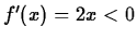 so
so  is decreasing for . Similarly, is increasing for
. This suggests the following procedure for determining where a
function is increasing or decreasing.
is decreasing for . Similarly, is increasing for
. This suggests the following procedure for determining where a
function is increasing or decreasing.
- Find the critical points of . Note that according to the
definition in the text, critical points of are points where either
is zero, the derivative doesn't exist, or endpoints of if
is defined on a finite interval .
- The critical points divide the domain of into subintervals
on which the sign of is constant. Check the sign of at one
interior point on each subinterval. If it is positive, is
increasing on that subinterval. If it is negative, is decreasing
on that subinterval.
The second derivative,  also provides
information about the shape of the curve in terms of what is called
concavity. Concavity can also be defined in several ways. Geometrically,
it can be said that the graph of is concave up near a point
if the tangent line at lies below the graph of on some
open interval containing and is concave up if the tangent line
lies above the graph of on some open interval containing
also provides
information about the shape of the curve in terms of what is called
concavity. Concavity can also be defined in several ways. Geometrically,
it can be said that the graph of is concave up near a point
if the tangent line at lies below the graph of on some
open interval containing and is concave up if the tangent line
lies above the graph of on some open interval containing
 . Algebraically, concavity is most often defined by saying that
is concave up on an interval if is increasing on and is
concave down on if is decreasing on . Using the theorem
above and remembering that
. Algebraically, concavity is most often defined by saying that
is concave up on an interval if is increasing on and is
concave down on if is decreasing on . Using the theorem
above and remembering that  is the derivative of gives the
following result.
is the derivative of gives the
following result.
This means that we can find where is concave up and concave down
using the same procedure on that we used on
. That is, we first find all of values of for which  , or
doesn't exist. Including the endpoints, if our domain is a
finite interval, these values of are the endpoints of distinct
subintervals on which the sign of is constant. Checking the sign
of at one point in the interior of each subinterval determines
the concavity of on that subinterval.
, or
doesn't exist. Including the endpoints, if our domain is a
finite interval, these values of are the endpoints of distinct
subintervals on which the sign of is constant. Checking the sign
of at one point in the interior of each subinterval determines
the concavity of on that subinterval.
Remember also that the second derivative can be helpful in determining
local maximums and local minimums. That is, if you find a critical
value, where or is undefined, then substitute the critical
value into the second derivative. If the second derivative is
positive, then there is a relative minimum there and if the second
derivative is negative, then there is a relative maximum there.
The Maple commands that are most useful are the ones for plotting
functions, taking derivatives, and solving equations. By plotting the
function and/or its derivatives, you can get a very good idea of where
it is increasing/decreasing and where it is concave up/concave
down. Then using the solve or fsolve commands
you can find the values of where or . Finally,
you can use Maple to check the signs of or in the interior
of the subintervals. The example below shows how you can use Maple to
find intervals where the function
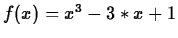 is increasing and
decreasing.
is increasing and
decreasing.
> f := x-> x^3-3*x+1;
> plot(f(x),x=-3..3);
> solve(D(f)(x)=0,x);
> D(f)(-2);
> D(f)(0);
> D(f)(2);
The plot helps to see how many critical values you have. The
solve command shows that there are critical values at  and
and  which means that the intervals can be broken up into
 ,
,  , and
, and  . Remember that if
solve doesn't work or doesn't find all critical values, you
can use the fsolve command specifying ranges for in which
to solve. Then chosing a point in each interval, we can see that the
value of the derivative is positive at
. Remember that if
solve doesn't work or doesn't find all critical values, you
can use the fsolve command specifying ranges for in which
to solve. Then chosing a point in each interval, we can see that the
value of the derivative is positive at  which implies that the
function is increasing on the interval . We can also
use the second derivative test to classify and as
relative maximum or relative minimum. See the Maple commands below to
help you do this.
which implies that the
function is increasing on the interval . We can also
use the second derivative test to classify and as
relative maximum or relative minimum. See the Maple commands below to
help you do this.
> D[1,1](f)(-1);
> f(-1);
> D[1,1](f)(1);
> f(1);
As you can see, the value of the second derivative at is
negative implying that  is a relative maximum. The value of
the second derivative at is positive which means that
is a relative maximum. The value of
the second derivative at is positive which means that  is a relative minimum.
- For the function
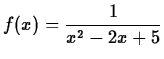 , find
the intervals on which is increasing and the intervals on which
it is decreasing.
, find
the intervals on which is increasing and the intervals on which
it is decreasing.
- For the function
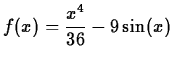 ,
,
- Plot over the interval
 .
.
- Find all critical values.
- Find corresponding
 values for each critical value.
- Classify each point as a relative maximum or a relative minimum
using the second derivative test.
- Find the absolute extrema for the function
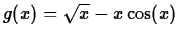 on the closed interval
 ![$[0,12]$](img44.png) .
.
Next: About this document ...
Up: lab_template
Previous: lab_template
William W. Farr
2002-10-01