These last two attempts at solving our problem use the worksheet from the previous section. You don't have to reload it.
Solution method 5 demonstrates what happens if the equations you want to solve are complicated and contain several parameters. Type in the command shown below.
> sol1 := solve({x(t)=30,y(t)=5},{t,theta});
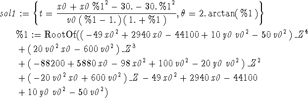
This is only a mild example of a Maple result that is not very useful,
but it contains some structures that are worth explaining. First
notice that the solutions for t and ![]() depend on an expression
called %1, which is defined at the bottom of the output region. Maple
does this simply to save space in the output. It notices that the
solution depends on this expression and saves space by writing the
expression only once and writing the solution in terms of this
expression.
depend on an expression
called %1, which is defined at the bottom of the output region. Maple
does this simply to save space in the output. It notices that the
solution depends on this expression and saves space by writing the
expression only once and writing the solution in terms of this
expression.
The other unfamiliar thing that appears in the output of this command
is a Maple RootOf structure. Maple uses RootOf(expr)
as a placeholder, where expr is a polynomial in ![]() and
RootOf(expr) stands for any root of the polynomial. For
example,
and
RootOf(expr) stands for any root of the polynomial. For
example, ![]() stands for either of the two roots
1 and -1 of
stands for either of the two roots
1 and -1 of ![]() . Maple always uses the variable
. Maple always uses the variable ![]() in
RootOf structures, so you should avoid using it for one of
your own labels.
in
RootOf structures, so you should avoid using it for one of
your own labels.
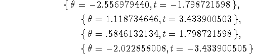
This is a little easier to see if we substitute the parameter values into the solution with the following command.
> subs(par_vals2,sol1);
What this is saying is that there is a solution to the equations for
each root of the polynomial in the RootOf structure. Given a
root, substituting it into the formulas for t and ![]() gives a
solution.
gives a
solution.
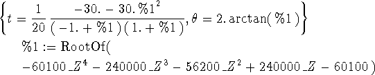
There are Maple commands that can be used to manipulate RootOf structures, but they are not usually needed in calculus. Instead, we take another approach to solve our problem. This is to substute the values of the parameters into the equations before invoking the solve command. A way to do it is shown below.
> solve(subs(par_vals2,{x(t)=30,y(t)=5}),{t,theta});