Subsections

• Purpose
• Background
  • Implicit Differentiation
  
  
• Exercises

Implicit Differentiation

Purpose

The purpose of this lab is to give you experience using Maple to compute derivatives of functions defined implicitly.

Background

Implicit Differentiation

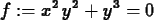
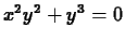
The implicitdiff command can be used to find derivatives of implicitly defined functions. Suppose we wanted to use implicit differentiation to find $$\frac{dy}{dx}$$ for the relation

$$x^2y^2+y^3=0$$

Then we first define our relation and give it a label for later use.

  > 
f:=x^2*y^2+y^3=0;

The syntax of the implicitdiff command is shown by the following example.

  > 
implicitdiff(f,y,x);

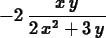
The result of the command is the implicit derivative, $$\frac{dy}{dx}$$. The syntax of this command is very similar to that of the diff command. The first argument is always the relation that you want to differentiate implicitly. We were careful to use an equation for this argument, but if you just give an expression for this argument, Maple assumes you want to set this expression equal to zero before differentiating. The second argument to the implicitdiff command is where you tell Maple what the dependent variable is. That is, by putting y here, we were saying that we were thinking of this relation as defining $y(x)$ and not $x(y)$. The remaining arguments to implicitdiff are for specifying the order of the derivative you want. See below for an example of finding the second derivative implicitly.

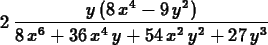
Second derivatives can also be taken with implicitdiff. The following command computes $$\frac{d^2y}{dx^2}$$.

  > 
implicitdiff(f,y,x,x);

To compute numerical values of derivatives obtained by implicit differentiation, you have to use the subs command. For example, to find the value of $$\frac{dy}{dx}$$ at the point $(1,-1)$ you could use the following command.

  > 
subs({x=1,y=-1},implicitdiff(f,y,x));

Sometimes you want the value of a derivative, but first have to find the coordinates of the point. More than likely, you will have to use the fsolve command for this. However, to get the fsolve command to give you the solution you want, you often have to specify a range for the variable. Being able to plot the graph of a relation can be a big help in this task, so we now describe the implicitplot command. This Maple command for plotting implicitly defined functions is in the plots package which must be loaded before using the command.

  > 
with(plots):

Here is an example of using this command to plot the hyperbola $x^2-y^2=1$. Note that you have to specify both an $x$ range and a $y$ range. This is because the implicitplot command works by setting up a grid inside the ranges you specify and then using the grid points as starting values in solving the relation numerically.

  > 
implicitplot(x^2-y^2=1,x=-3..3,y=3..3);

To get a good graph with this command, you usually have to experiment with the ranges. For example the following command

  > 
implicitplot(f,x=-1..1,y=1..2);

produces an empty plot. The reason is simply that there are no solutions to $x^2y^2+y^3 = 0$ with $y > 0$. This is easy to see if you rewrite the equation as $x^2y^2= -y^3$ and recognize that both sides of the equation must be nonnegative. Usually a good strategy to follow is to start with fairly large ranges, for example $-10$ to $10$ for both variables, and then refine them based on what you see.

Here is an example of finding the two points on the graph of the relation $x^2+y^2-y+x/2=2$ where the tangent line is horizontal. The first step is to plot the graph using implicitdiff so that you can approximately the locations of the points where the tangent line is horizontal. Then you use the fsolve command to find the points in question.

  > 
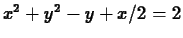
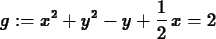
g := x^2+y^2-y+x/2=2;

  > 
implicitplot(g, x=-2..2,y=-2..2.5);

Looking at the plot, the horizontal tangents occur approximately at the two points $(-1/4,2)$ and $(-1/4,-1)$. To find them more exactly, we can use the fsolve command. Such points have to satisfy two conditions. The have to be on the graph and the slope has to be zero there. The following commands first compute the derivative implicitly and then find the two points using fsolve. The exact ranges you use for the fsolve command are not crucial, but you should choose them so that each includes exactly one of the solution points. If you don't do this, the fsolve command may fail to find a solution or may only find one solution.

  > 
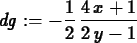
dg := implicitdiff(g,y,x);

  > 
fsolve({g,dg=0},{x,y},x=-1..0,y=1.5..2.5);

  > 
fsolve({g,dg=0},{x,y},x=-1..0,y=-1.5..-0.5);

The implictiplot command can also have problems if the relation in question has solution branches that cross or are too close together. For example, try the following command.

  > 
implicitplot(f,x=-1..1,y=-1..0);

For $y$ less than about $-0.2$, you should see the two smooth curves. However, for values of $y$ closer to zero the two curves become jagged. To understand this, we need to take a closer look at the relation we tried to plot. The key is to notice that we can factor out $y^2$ and write our relation as follows.

$$y^2 (x^2+y)$$

This makes it clear that the graph of the relation really has two pieces: $y=0$ and $y=-x^2$. These two curves intersect at the origin, which explains why implicitplot has problems there.

As our last example, consider the relation 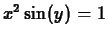$x^2 \sin(y)=1$. Try the following commands to see what a part of the graph of this relation looks like.

  > 
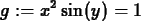
g := x^2*sin(y)=1;

  > 
implicitplot(g,x=-4..4,y=-10..10);

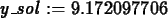
Suppose you were asked to find the slope of the graph of this relation at $x=2$, but you were only given that the value of $y$ was about 9. Using the plot, it is relatively easy to find this derivative by first using fsolve to find the $y$ value and then substituting to into the formula for the derivative. Note the use of a label so we can use the value of $y$ in the next command.

  > 
y_sol := fsolve(subs(x=2,g),y,y=8..10);

  > 
evalf(subs({x=2,y=y_sol},implicitdiff(g,y,x
)));

Exercises

1. Find the slope of the graph of $x^2y+y^2+2x-3=0$ at the point $(3/2,0)$. Supply a plot of the graph that includes the point in question.

2. For the relation $x^2y+y^2+2x-3=0$ from the first exercise, find the coordinates of the three points on the graph where the tangent line is horizontal.

3. For the relation $x^2-y^2+2y = 4$, find $$\frac{d^2y}{dx^2}$$ at the point $(2,2)$.

4. Consider the relation
   
   $$\frac{x^2+y}{1-xy} = 2$$
   
   
   1. Use implicit differentiation to find the derivative $dy/dx$.
   2. Solve the relation for $y$ and then compute $dy/dx$ directly.
   3. Compare your two results. Can you show that they are equal?