Subsections

• Purpose
• Background
  • Introduction
  • Definite and indefinite integrals with Maple
  • Applications - averages and centroids
  
  
• Exercises

The Definite Integral

Purpose

The purpose of this lab is to introduce you to Maple commands for computing definite and indefinite integrals.

Background

Introduction

There are two main ways to think of the definite integral. The easiest one to understand is as a means for computing areas (and volumes). The second way the definite integral is used is as a sum. That is, we use the definite integral to ``add things up''. Here are some examples.

• Computing net or total distance traveled by a moving object.
• Computing average values, e.g. centroids and centers of mass, moments of inertia, and averages of probability distributions.

This lab is intended to introuduce you to Maple commands for computing integrals, including applications of integrals.

Definite and indefinite integrals with Maple

The basic Maple command for computing definite and indefinite integrals is the int command. The syntax is very similar to that of the leftsum and rightsum commands, except you don't need to specify the number of subintervals. Suppose you wanted to compute the following definite integral with Maple.

$$\int_{0}^{4} x^2 \, dx$$

The command to use is shown below.

> int(x^2,x=0..4);

Notice that Maple gives an exact answer, as a fraction. If you want a decimal approximation to an integral, you just put an evalf command around the int command, as shown below.

> evalf(int(x^2,x=0..4));

To compute an indefinite integral with Maple, you just leave out the range for the limits of integration, as shown below.

> int(x^2,x);

Note that Maple does not include a constant of integration.

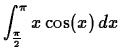
You can also use the Maple int command with functions or expressions you have defined in Maple. For example, suppose you wanted to find area under the curve of the function $f(x)=x \sin(x)$ on the interval $[0,\pi]$. Then you can define this function in Maple with the command

> f := x -> x*sin(x);

and then use this definition as shown below.

> int(f(x),x=0..Pi);

You can also simply give the expression corresponding to $f(x)$ a label in Maple, and then use that label in subsequent commands as shown below. However, notice the difference between the two methods. You are urged you to choose one or the other, so you don't mix the syntax up.

> p := x*sin(x);
> int(p,x=0..Pi);

Applications - averages and centroids

If a function $f$ is integrable over an interval $[a,b]$, then we define the average value of $f$, which we'll denote as $\bar{f}$, on this interval to be

$$\bar{f} = \frac{1}{b-a} \int_{a}^{b} f(x) \, dx$$

Note that the average value is just a number. For example, suppose you wanted to compute the average value of the function $s(t) = -16t^2+100t$ over the interval $1 \leq t \leq 5$. The following Maple command would do the job.

> int(-16*t^2+100*t,t=1..5)/(5-1);

It is also easy to use Maple to compute centroids and centers of mass. For example, suppose you wanted to compute the coordinates of the centroid of the region bounded above by the curve $g(x) = -3x^2+3x+36$ and below by the $x$ axis over the interval $-3 \leq x \leq 4$. The first thing to do is to plot the region.

> q := -3*x^2+3*x+36;
> plot(q,x=-3..4);

Once you have plotted the region, you can compute the area with the following command. Note the use of a label, since we'll use the area later.

> area := int(q,x=-3..4);

Once we have the area, we can compute $\bar{x}$ and $\bar{y}$ as follows.

> x_bar := int(x*q,x=-3..4)/area;
> y_bar := int(q^2,x=-3..4)/(2*area);

Exercises

1. Use Maple to compute the following definite integrals.
   1. $$\int_{-2}^{4} (x^2+3x+1)^2(x^3+1) \, dx$$
   2. $$\int_{\frac{\pi}{2}}^{\pi} x \cos(x) \, dx$$

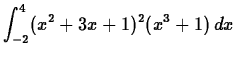
2. Find the area of the region bounded above by $y=2x+1$ and below by 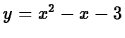$y=x^2-x-3$. Include a plot of the region.

3. Find the centroid of the region from the previous exercise.

4. Suppose the velocity in feet per second of a particle moving in one dimension is given by
   
   $$v(t) = 110-4t + 15 \cos(3t)$$
   
   
   where $t$ is the time in seconds.
   1. Find the average velocity of the particle over the interval $0 \leq t \leq 3$.
   2. Assuming that the particle was at the origin at $t=0$, determine the position of the particle at $t=3$.