Rectangular Approximation

In these simple approximation schemes, the area above each subinterval is approximated by the area of a rectangle, with the height of the rectangle being chosen according to some rule. The rules we will be concerned with are as follows.

left endpoint rule

The height of the rectangle is the value of the function f(x) at the left-hand endpoint of the subinterval.

right endpoint rule

The height of the rectangle is the value of the function f(x) at the right-hand endpoint of the subinterval.

The Maple student package has commands for visualizing these two rectangular area approximations. To use them, you first must load the student package via the with command. Then try the commands given below. Make sure you understand the differences between the two different rectangular approximations.

  > with(student):

  > f:=x-> x^2 ;

  > rightbox(f(x),x=0..4);

  > leftbox(f(x),x=0..4);

There are also Maple commands leftsum and rightsum to sum the areas of the rectangles, see the examples below. Note the use of evalf to obtain numerical answers.

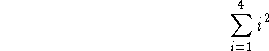
  > rightsum(f(x),x=0..4);

  > evalf(rightsum(f(x),x=0..4));

  > evalf(rightsum(x,x=0..2));

Unless specified, Maple will break the given interval into four subintervals. Below are some examples of how to change the number of subintervals used in the approximation.

  > evalf(rightsum(x,x=0..2,10));

  > evalf(rightsum(x,x=0..2,20));

  > evalf(rightsum(x,x=0..2,100));