Subsections

• Introduction
• Background
• Graphs of Solids of Revolution
• Volumes of Solids of Revolution
• Exercises

Solids of Revolution

Introduction

The purpose of this lab is to use Maple to study solids of revolution. Solids of revolution are created by rotating curves in the x-y plane about an axis, generating a three dimensional object. The specific properties of them that we wish to study are their graph and volume.

Background

So far we have used the integral mainly to to compute areas of plane regions. It turns out that the definite integral can also be used to calculate the volumes of certain types of three-dimensional solids. The class of solids we will consider in this lab are called Solids of Revolution because they can be obtained by revolving a plane region about an axis.

Graphs of Solids of Revolution

As a simple example, consider the graph of the function $f(x) = x^2+1$ for $-2 \leq x \leq 2$ which you can plot on Maple:

> f := x-> x^2+1;
> plot(f(x),x=-2..2);

If we take the region between the graph and the x-axis and revolve it about the x-axis, we obtain a 3-D solid.

To plot this solid of revolution using Maple, the revolve command can be used. All of the procedures described in this lab are part of the CalcP7 package, which must be loaded first. The syntax for revolve when revolving $f(x)$ about the $x$-axis over the interval $a \leq x \leq b$ is:

> revolve(f(x),x=a..b);

If you revolve the area under the graph of $f(x)$ for $a \leq x \leq b$ about the $x$-axis, the volume is given by

$$\pi \int_{a}^{b} (f(x))^2 \, dx.$$

The integral formula given above for the volume of a solid of revolution comes, as usual, from a limit process. Recall the rectangular approximations we used for plane regions. If you think of taking one of the rectangles and revolving it about the x-axis, you get a disk whose radius is the height $h$ of the rectangle and thickness is $\Delta x$, the width of the rectangle. The volume of this disk is $\pi h^2 \Delta x$. If you revolve all of the rectangles in the rectangular approximation about the x-axis, you get a solid made up of disks that approximates the volume of the solid of revolution obtained by revolving the plane region about the x-axis.

To help you visualize this approximation of the volume by disks, the LeftDisk procedure has been written. The syntax for this command is similar to that for revolve, except that the number of subintervals must be specified. The examples below produce approximations with five and ten disks. The last example produces the exact solid of revolution.

> with(CalcP7):
> f := x -> x^2+1;
> LeftDisk(f(x),x=-2..2,5);
> LeftDisk(f(x),x=-2..2,10);
> revolve(f(x),x=-2..2);

The revolve command has optional arguments. A third argument can be added to specify a different axis of revolution. For instance, we may want to revolve the graph of $f(x)$ about the line $y=-2$ instead of the default $y=0$. Also, the nocap argument can speed up the plotting process by only plotting the surface generated by revolving the curve instead of solid generated by revolving the area. Below is an example of what the 3-D solid looks like when revolving $f(x)$ about the line $y=-2$.

> revolve(f(x),x=-2..2,y=-2,nocap);

You can also plot a solid of revolution formed by revolving the area between two functions. Try the following examples.

> plot({5,x^2+1},x=-2..2);
> revolve({5,x^2+1},x=-2..2);

Volumes of Solids of Revolution

As stated earlier, the volume of the solid obtained by revolving the region under the graph of $f(x)$, above the $x$-axis, over the interval $a \leq x \leq b$ is given by

$$\pi \int_a^b f(x)^2 \, dx.$$

Therefore, the volume of the solid obtained by revolving the region between the graph of $f(x) = x^2+1$ and the $x$-axis about the $x$-axis can be determined from the integral $$\pi \int_{-2}^2 (x^2+1)^2 \, dx$$.

In order to calculate the volume of a solid of revolution, you can either use the int command implementing the formula above or use the Maple procedure RevInt which sets up the integral for you. The Maple commands evalf and value can be used to obtain a numerical or analytical value. Approximations to the volume of the solid of revolution can be found using the LeftInt. Try the examples below to see the different types of output.

> Pi*int(f(x)^2,x=-2..2);
> evalf(Pi*int(f(x)^2,x=-2..2));
> RevInt(f(x),x=-2..2);
> value(RevInt(f(x),x=-2..2));
> evalf(RevInt(f(x),x=-2..2));
> evalf(LeftInt(f(x),x=-2..2,50));

Exercises

1. For the function $$f(x) = \frac{3+x\cos(2x)}{x^2+1}$$ over the interval $-2 \leq x \leq 2$,
   1. Plot $f(x)$ over the given interval.
   2. Plot the approximation of the solid of revolution using $LeftDisk$ with 12 disks.
   3. Plot the solid formed by revolving $f(x)$ about the $x$-axis.
   4. Plot the solid formed by revolving $f(x)$ about the line $y=-1$.
   5. Find the exact volume of the solid of revolution about the $x$-axis using the integral formula.
   6. Find the exact volume of the solid of revolution using the RevInt command and label your output exact.
   7. Find the minimum number of subintervals needed to approximate the volume of the solid of revolution about the $x$-axis using LeftInt with error no greater than 0.01.

2. What function's graph can be revolved about the $x$-axis to obtain a sphere of radius $R$? Use this function and the RevInt command to prove that the volume of a sphere is $$\frac{4}{3} \pi R^3$$.

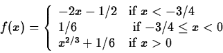
3. Six years ago, Kevin Nordberg and James Rush (both class of '98) were asked to design a drinking glass by revolving a suitable function about the $x$ axis. Here is the function they came up with.

   
   

   $$f(x) = \left\{ \begin{array}{ll} -2x-1/2 & \mbox{if $x < -3/... ...< 0$} \\ x^{2/3}+1/6 & \mbox{if $x > 0$} \end{array}\right.$$
   
   
   They obtained the shape of their glass by revolving this function about the $x$ axis over the interval $[-1,2]$. The Maple command they used to define this function is given below.

   > f := x -> piecewise(x<-3/4,-2*x-1/2,x<0,1/6,x^(2/3)+1/6);
   

   Plot this function (without revolving it) over the interval $[-1,2]$ and identify the formula for each part of the graph. Then, revolve this function about the $x$ axis over the same interval and comment on the glass Kevin and Jim designed. Finally, compute the volume of the part of this glass that could be filled with liquid, assuming the stem is solid. (Hint - your integral will involve only one of the formulas used to define the function.)