Two widely used rules for approximating areas are the trapezoidal rule and Simpson's rule. To motivate the new methods, we recall that rectangular rules approximated the function by a horizontal line in each interval. It is reasonable to expect that if we approximate the function more accurately inside each interval then a more efficient numerical scheme will follow. This is the idea behind the trapezoidal and Simpson's rules. Here the trapezoidal rule approximates the function by a suitably chosen (not necessarily horizontal) line segment. The function values at the two points in the interval are used in the approximation. While Simpson's rule uses a suitably chosen parabolic shape (see Section 4.6 of the text) and uses the function at three points.
The Maple student package has commands trapezoid and simpson that implement these methods. The command syntax is very similar to the rectangular approximations. See the examples below. Note that an even number of subintervals is required for the simpson command and that the default number of subintervals is n=4 for both trapezoid and simpson.
> with(student):
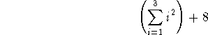
> trapezoid(x^2,x=0..4);
> evalf(trapezoid(x^2,x=0..4));
![]()
> evalf(trapezoid(x^2,x=0..4,10));
![]()
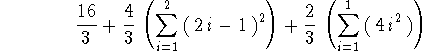
> simpson(x^2,x=0..4);
> evalf(simpson(x^2,x=0..4));
![]()
> evalf(simpson(x^2,x=0..4,10));
![]()