Subsections

• Introduction
• Rectangular Approximations
• Accuracy
• Exercises

Rectangular Approximations to Integrals

Introduction

The purpose of this lab is to acquaint you with some rectangular approximations to integrals.

Rectangular Approximations

Integration, the second major theme of calculus, deals with areas, volumes, masses, and averages such as centers of mass and gyration. In lecture you have learned that the area under a curve between two points $a$ and $b$ can be found as a limit of a sum of areas of rectangles which approximate the area under the curve of interest. Not all ``area finding'' problems can be solved using analytical techniques. The Riemann sum definition of area under a curve gives rise to several numerical methods which can approximate the area of interest with great accuracy.

Suppose $f(x)$ is a non-negative, continuous function defined on some interval $[a,b]$. Then by the area under the curve $y=f(x)$ between $x=a$ and $x=b$ we mean the area of the region bounded above by the graph of $f(x)$, below by the $x$-axis, on the left by the vertical line $x=a$, and on the right by the vertical line $x=b$. All of the numerical methods in this lab depend on subdividing the interval $[a,b]$ into subintervals of uniform length.

In these simple rectangular approximation methods, the area above each subinterval is approximated by the area of a rectangle, with the height of the rectangle being chosen according to some rule. In particular, we will consider the left, right and midpoint rules.

The Maple student package has commands for visualizing these three rectangular area approximations. To use them, you first must load the package via the with command. Then try the three commands given below to help you understand the differences between the three different rectangular approximations. Note that the different rules choose rectangles which in each case will either underestimate or overestimate the area.

> with(student):
> rightbox(x^2,x=0..4,3);
> leftbox(x^2,x=0..4,16);
> middlebox(x^2,x=0..4,10);

There are also Maple commands leftsum, rightsum, and middlesum to sum the areas of the rectangles, see the examples below. Note the use of evalf to obtain the desired numerical answers.

> rightsum(x^2,x=0..4);
> evalf(rightsum(x^2,x=0..4,3));
> evalf(leftsum(x^2,x=0..4,16));
> evalf(middlesum(x^2,x=0..4,10));

Accuracy

It should be clear from the graphs that adding up the areas of the rectangles only approximates the area under the curve. However, by increasing the number of subintervals the accuracy of the approximation can be improved. One way to measure how good the approximation is is the absolute error, which is the difference between the actual answer and the estimated answer. Later on in the course, you will learn techniques for finding the exact answer. Approximations, however, are important because exact answers cannot always be found.

All of the Maple commands described so far in this lab can include a third argument to specify the number of subintervals. The default is 4 subintervals. The example below approximates the area under $y=x^2$ from $x=0$ to $x=4$ using the rightsum command with 50, 100, 320 and 321 subintervals. As the number of subintervals increases, the approximation gets closer and closer to the exact answer. You can see this by assigning a label to the approximation, assigning a label to the exact answer $(4^3/3)$ and taking their difference. The closer you are to the actual answer, the smaller the difference. The example below shows how we can use Maple to approximate this area with an absolute error no greater than 0.1.

> exact := 4^3/3;
> estimate := evalf(rightsum(x^2,x=0..4,50));
> evalf(abs(exact-estimate));
> estimate := evalf(rightsum(x^2,x=0..4,100));
> evalf(abs(exact-estimate));
> estimate := evalf(rightsum(x^2,x=0..4,320));
> evalf(abs(exact-estimate));
> estimate := evalf(rightsum(x^2,x=0..4,321));
> evalf(abs(exact-estimate));

Exercises

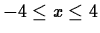
1. Consider the function 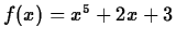$f(x)=x^5+2x+3$ on the interval $[-1,2]$

   A)

   Use the rightbox command to plot the rectangular approximation of the area above the $x-axis$ and under $f(x)$ with twelve rectangles.

   B)

   Use the leftbox command to plot the rectangular approximation of the area above the $x-axis$ and under $f(x)$ with twelve rectangles.

   C)

   Use the middlebox command to plot the rectangular approximation of the area above the $x-axis$ and under $f(x)$ with twelve rectangles.

   D)

   Which graph gives the best approximation to the area and give your reasoning.

2. Plot the function 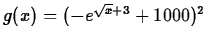$g(x)=(-e^{\sqrt{x}+3}+1000)^2$ on the interval $[0,15]$ with seven rectangles determined by the right-endpoint rule. Then plot the function with the left-endpoint rule.

   A)

   Which rule underestimates the area for this function? Will this rule always underestimate area for any function? Why?

   B)

   Which rule overestimates the area for this function? Will this rule always underestimate area for any function? Why?

3. The area under 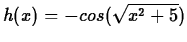$h(x)=-cos(\sqrt{x^2+5})$ above the $x-axis$ over the interval $-4\leq x \leq 4$ accurate to ten decimal places is 6.0632791021.

   A)

   Plot $h(x)$ over the given interval.

   B)

   Use the command rightsum to find the minimum number of subintervals needed to approximate the area with error no greater than 0.001.

   C)

   Use the command middlesum to find the minimum number of subintervals needed to approximate the area with error no greater than 0.001.

   D)

   Which method requires the least number of subintervals.