Subsections

• Purpose
• Background
• Accuracy and Tolerance
• Maple Commands
• Exercises

Taylor Polynomials

Purpose

The purpose of this lab is to use Maple to introduce you to Taylor polynomial approximations to functions, including some applications.

Background

The idea of the Taylor polynomial approximation of order $n$ at $x=a$, written $P_n(x,a)$, to a smooth function $f(x)$ is to require that $f(x)$ and $P_n(x,a)$ have the same value at $x=a$. Furthermore, their derivatives at $x=a$ must match up to order $n$. For example the Taylor polynomial of order three for $\sin(x)$ at $x=0$ would have to satisfy the conditions

$$\begin{array}{ccccc} P_3(0,0) & = & \sin(0) & = & 0\\ P_3'(0... ...0) & = & 0 \\ P_3'''(0,0) & = & -\cos(0) & = & -1 \end{array}$$

You should check for yourself that the cubic polynomial satisfying these four conditions is

$$P_3(x,0) = x - \frac{1}{6} x^3.$$

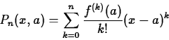
The general form of the Taylor polynomial approximation of order $n$ to $f(x)$ is given by the following

Theorem 1   Suppose that $f(x)$ is a smooth function in some open interval containing $x=a$. Then the $n$th degree Taylor polynomial of the function $f(x)$ at the point $x=a$ is given by

$$P_n(x,a) = \sum_{k=0}^{n} \frac{f^{(k)}(a)}{k!} (x-a)^k$$

$$= f(a) + f'(a)(x-a) + \frac{f''(a)}{2}(x-a)^2 + \cdots + \frac{f^{(n)}(a)}{n!} (x-a)^n$$

We will be seeing this formula a lot, so it would be good for you to memorize it now! The notation $f^{(k)}(a)$ is used in the definition to stand for the value of the $k$-th derivative of $f$ at $x=a$. That is, $f^{(1)}(a) = f'(a)$, $f^{(3)}(a) = f'''(a)$, and so on. By convention, $f^{(0)}(a) = f(a)$. Note that $a$ is fixed and so the derivatives $f^{(k)}(a)$ are just numbers. That is, a Taylor polynomial has the form

$$\sum_{k=0}^{n} a_k (x-a)^k$$

which you should recognize as a power series that has been truncated.

Accuracy and Tolerance

To measure how well a Taylor Polynomial approximates the function over a specified interval $[c,d]$, we define the tolerance $Tol$ of $P_n(x,a)$ to be the maximum of the absolute error

$$\mid f(x)- P_n(x,a) \mid$$

over the interval $[c,d]$. The Getting started worksheet has examples of how to compute and plot the absolute error.

Maple Commands

To use the Taylor and TayPlot commands you need to load the CalcP7 package. First you need to go to the dtterm window and type

cp ~bfarr/.mapleinit ~

If nothing happens when you press enter then you did it correctly. Otherwise try again. This will give you access to the package and therefore you can call it up on the Maple screen with the command

>with(CalcP7);

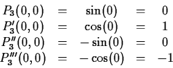
The exponential function can be approximated at a base point zero with a polynomial of order four using the following command.

>Taylor(exp(x),x=0,4);

You might want to experiment with changing the order. To see $f(x) = \exp(x)$ and its fourth order polynomial use

>TayPlot(exp(x),x=0,{4},x=-4..4);

This plots the exponantial and three approximating polynomials.

>TayPlot(exp(x),x=0,{2,3,4},x=-2..2);

Notice that the further away from the base point, the further the polynomial diverges from the function. the amount the polynomial diverges i.e. its error, is simply the difference of the function and the polynomial.

>plot(abs(exp(x)-Taylor(exp(x),x=0,3)),x=-2..2);

This plot shows that in the domain x from -2 to 2 the error around the base point is zero and the error is its greatest at x = 2 with a difference of over one. You can experiment with the polynomial orders to change the accuracy. If your work requires an error of no more than 0.2 within a given distance of the base point then you can plot your accuracy line y = 0.2 along with the difference of the function and the Taylor approximation polynomial.

>plot([0.2,abs(exp(x)-Taylor(exp(x),x=0,3))],x=-2..2,y=0..0.25);

We knew this would have some of its error well above 0.2. Change the order from three to four. As you can see there are still some values in the domain close to x = 2 whose error is above 0.2. Now try an order of 5. Is the error entirely under 0.2 between x = -2 and x = 2? Larger orders will work as well but order five is the minimum order that will keep the error under 0.2 within the given domain.

Exercises

1. For the following functions and base points, determine what minimum order is required so that the Taylor polynomial approximates the function to within a tolerance of $0.1$ over the given interval.
   1. $f(x) = \sin(x)$, base point $a=0$, interval $[0 ,6\pi ]$.
   2. $f(x) = 1/(1-x)$, base point $a=0$, interval $[-0.9,0.9]$.
   3. $f(x) = x/(x+1)^2$, base point $a=1$, interval $[-0.5,2.5]$.
   4. $f(x) = x^4\ln(x+1)$,base point $a=2$, interval $[0.5,3.5]$.

2. For the function, $f(x) = 1/(x-1)$, use the TayPlot command to plot the function and multiple Taylor polynomial approximations of various orders with base point $a=0$ on the same graph over the interval $-2.5 \leq x \leq 0$; use a y-range from -3 to 3. If you increase the order of the Taylor polynomial, can you get a good approximation at $x=-1.2$? Can you make a good guess at the radius of convergence of the Taylor series for $f$?

   A theorem from complex variables says that the radius of convergence of the Taylor series of a function like $f$ is the distance between the base point ($a=0$ in this case) and the nearest singularity of the function. By singularity, what is meant is a value of $x$ where the function is undefined. Where is $f$ undefined? Is the distance between this point and the base point consistent with your guess of the radius of convergence from the plot?