The purpose of this lab is to use Maple to introduce you to a number of useful commands for working with vectors, including some applications. The commands come from the Maple linalg and CalcP7 packages which must be loaded before any of its commands can be used.
cp /math/calclab/MA1023/Vector_start2.mws ~/My_Documents
You can copy the worksheet now, but you should read through the lab before you load it into Maple. Once you have read through the exercises, start up Maple, load the worksheet, and go through it carefully. Then you can start working on the exercises.
For this lab, we will assume that we have a vector-valued function ![]() that gives the position at time
that gives the position at time ![]() of a moving point
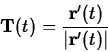
of a moving point ![]() in the plane. The velocity of this point is given by the derivative
in the plane. The velocity of this point is given by the derivative ![]() and the acceleration is given by the second derivative,
and the acceleration is given by the second derivative, ![]() . In many applications of curvilinear motion, we need to know the magnitude of the velocity, or the speed. This is easy to compute - just take the magnitude
. In many applications of curvilinear motion, we need to know the magnitude of the velocity, or the speed. This is easy to compute - just take the magnitude ![]() . If you think of the speed as the rate of change of distance along the curve, and recall that arc length is distance measured along the curve, then you have the following interpretation of the speed
. If you think of the speed as the rate of change of distance along the curve, and recall that arc length is distance measured along the curve, then you have the following interpretation of the speed
>PLOT3D(POLYGONS([[-3,-15,-1],[0.80477,-1.597614,8.7928429],[7,13,15],
[3.1952286,-0.40238569,5.207157]]),AXESSTYLE(NORMAL),AXESLABELS(x,y,z)
,VIEW(-10..10,-20..20,-1..20));
>PLOT3D(POLYGONS([[0,0,0],[3,0,0],[3,10,0],[0,10,0]],
[[0,0,0],[0,10,0],[0,10,4],[0,0,4]],[[3,0,0],[3,10,0],
[3,10,4],[3,0,4]],[[0,0,0],[3,0,0],[3,0,4],[0,0,4]],
[[0,10,0],[3,10,0],[3,10,4],[0,10,4]],[[0,0,4],[3,0,4],
[3,10,4],[0,10,4]]),AXES(NORMAL), COLOR(ZHUE),
VIEW(0..10,0..10,0..10),AXESLABELS(x,y,z));