Subsections

• Purpose
• Background
• Defining parametric curves and vector valued functions simply in Maple
• Plotting and animating curves in the plane
  • Derivatives and the slope
  
  
• Exercises

Parametric Curves in the Plane

Purpose

The purpose of this lab is to introduce you to curve computations using Maple for parametric curves and vector-valued functions in the plane.

Background

By parametric curve in the plane, we mean a pair of equations $x=f(t)$ and $y=g(t)$ for $t$ in some interval $I$. A vector-valued function in the plane is a function $\mathbf{r}(t)$ that associates a vector in the plane with each value of $t$ in its domain. Such a vector valued function can always be written in component form as follows,

$$\mathbf{r}(t) = f(t) \mathbf{i} + g(t) \mathbf{j}$$

where $f$ and $g$ are functions defined on some interval $I$. From our definition of a parametric curve, it should be clear that you can always associate a parametric curve with a vector-valued function by just considering the curve traced out by the head of the vector.

Defining parametric curves and vector valued functions simply in Maple

The easiest way to define a vector function or a parametric curve is to use the Maple list notaion with square brackets[]. Strictly speaking, this does not define something that Maple recognizes as a vector, but it will work with all of the commands you need for this lab.

>f:=t->[2*cos(t),2*sin(t)];

You can evaluate this function at any value of t in the usual way.

>f(0);

This is how to access a single component. You would use f(t)[2] to get the second component.

>f(t)[1]

Plotting and animating curves in the plane

The ParamPlot command is in the CalcP package so you have to load it first. If you get an error from this command, ask for help right away.

>with(CalcP7);

The ParamPlot command produces an animated plot. To see the animation, execute the command and then click on the plot region below to make the controls appear in the Context Bar just above the worksheet window.

>g:=t->[t,t^2];
>ParamPlot(g(t),t=-2..2);

You can use the VPlot command as shown below. Note that this command does not show the direction of the plot with respect to t.

>VPlot([t^2,t^3-t],t=-1.5..1.5);

Derivatives and the slope

The graph of a parametric curve may not have a slope at every point on the curve. When the slope exists, it must be given by the formula from class.

$$\frac{dy}{dx} = \frac{\frac{dy}{dt}}{\frac{dx}{dt}}$$

It is clear that this formula doesn't make sense if $$\frac{dx}{dt}= 0$$ at some particular value of $t$. If $$\frac{dy}{dt} \neq 0$$ at that same value of $t$, then it turns out the graph has a vertical tangent at that point. If both $$\frac{dx}{dt}$$ and $$\frac{dy}{dt}$$ are zero at some value of $t$, then the curve often doesn't have a tangent line at that point. What you see instead is a sharp corner, called a cusp. To find the derivative of each component of the parametric equation remember to use the [ ] at the end of the command. $\frac{dy}{dt}$ is:

>diff(g(t),t)[2];

$\frac{dx}{dt}$ is:

>diff(g(t),t)[1];

To get the derivative, divide the two: $\frac{dy}{dx}$ is:

>m:=diff(g(t),t)[1]/diff(g(t),t)[2];

Exercises

1. Enter the following two parametrization as functions.
   
   $$r_1(t)=(5\cos(t)+\cos(5t)){\bf i}+(5\sin(t)-\sin(5t)){\bf j}$$
   
   
   
   
   $$r_2(t)=4\cos(3t){\bf i}+4\sin(2t){\bf j}$$
   
   
   For $0 \leq t \leq 2\pi$ animate the two functions then animate them agaim after doubling the angles.Describe what effect doubling the angle has on the animation.

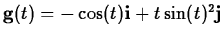
2. Enter the curve $\mathbf{j}(t) = (3t-1)\mathbf{i} + (2t^3-4)\mathbf{j}$

   A)

   For $-1 \leq t \leq 1$, plot the graph of $\mathbf{j}(t)$.

   B)

   Calculate the slope of $\mathbf{j}(t)$.

   C)

   Calculate the point at $t = 0$ and calculate the slope at the same t.

   D)

   Calculate the point at $t = \frac{1}{3}$ and calculate the slope at the same t.

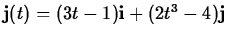
3. Enter the parametric equation $\mathbf{g}(t) = -\cos(t) {\bf i} + t\sin(t)^2 {\bf j}$.

   A)

   Plot the parameterization on the domain $-2\pi \leq t \leq 2\pi$

   B)

   find $\frac{dy}{dx}$

   C)

   Plot the numerator of the slope ($\frac{dy}{dt}$) - use the regular plot command.Then plot the denominator of the slope ($\frac{dx}{dt}$).

   D)

   Keeping your work clearly organized - use fsolve commands to find where the numerator equals zero.Then find where the denominator equals zero. (The plots from part C should tell you how many solutions to look for)

   E)

   At what t-values are there horizontal tangents?

   F)

   At what t-values are there vertical tangents?

   G)

   At what t-values are there cusps?