Suppose  is a smooth function, that is, it has derivatives of all orders.
Examples of such functions are polynomials and the transcendental
functions
is a smooth function, that is, it has derivatives of all orders.
Examples of such functions are polynomials and the transcendental
functions  ,
,  , and the trigonometric functions
 and
and  .
Polynomials are simple to do calculations with, but it isn't so
obvious how your calculator or a computer does
calculations with functions like
.
Polynomials are simple to do calculations with, but it isn't so
obvious how your calculator or a computer does
calculations with functions like  and
and  . In this lab we
will start to investigate a method for approximating smooth functions
with polynomials. Calculators and computers actually use related, but more
sophisticated, methods to approximate the values of transcendental
and trigonometric functions.
. In this lab we
will start to investigate a method for approximating smooth functions
with polynomials. Calculators and computers actually use related, but more
sophisticated, methods to approximate the values of transcendental
and trigonometric functions.
To help you understand where the polynomial approximations come from,
recall the linear approximation  to
to  at x=a, which
had the following properties:
at x=a, which
had the following properties:
 at x=a. That is,
  ;
;
 was equal to
  .
.

Recall that the linear approximation  was the straight line
tangent to
was the straight line
tangent to  . That is, it went through the point
  and
had slope
and
had slope  , the derivative of
  at x=a.
For example, suppose  and we choose a=0. To
compute the linear approximation to
and we choose a=0. To
compute the linear approximation to  at x=0, we need two
numbers:
at x=0, we need two
numbers:  and
and  . Plugging these
two numbers into the formula gives the answer
. Plugging these
two numbers into the formula gives the answer

If you plotted the linear approximation on the same graph as the
function  , you would see that the linear approximation is
tangent to the function at x=0.
, you would see that the linear approximation is
tangent to the function at x=0.
Changing the value of the base point a results in a different linear
function. For
example, setting the value  produces the linear approximation

which is tangent to  at
at  .
.
The linear approximation is usually a pretty good approximation to the
function  for
values of x that are very close to the base point a. It often
happens, though, that a better approximation is needed. One approach
that usually works is to use a higher order polynomial, for example a
quadratic polynomial, to approximate the function
for
values of x that are very close to the base point a. It often
happens, though, that a better approximation is needed. One approach
that usually works is to use a higher order polynomial, for example a
quadratic polynomial, to approximate the function  .
.
A way of
defining a quadratic polynomial that builds on our definition of the
linear approximation is given below. Simply put, we require that the
quadratic polynomial go through the point  , and have the
same first and second derivatives as
, and have the
same first and second derivatives as  at the point
x=a. Polynomial approximations defined
in this way turn out to
be very useful in a lot of different applications, and are referred to
as Taylor polynomials.
at the point
x=a. Polynomial approximations defined
in this way turn out to
be very useful in a lot of different applications, and are referred to
as Taylor polynomials.
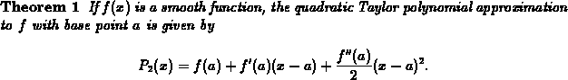
Given a function  and a base point a, the quadratic Taylor
polynomial approximation can always be obtained by substituting into
the three equations in the definition above and solving for the values
of the coefficients A, B, and C. For example, suppose
and a base point a, the quadratic Taylor
polynomial approximation can always be obtained by substituting into
the three equations in the definition above and solving for the values
of the coefficients A, B, and C. For example, suppose
 and we choose
  . Then subsituting into the three
equations in the definition produces the following equations.
. Then subsituting into the three
equations in the definition produces the following equations.
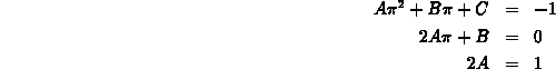
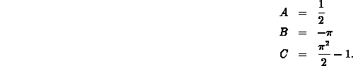
Solving these equations is straightforward; just start with the third equation and work your way back, leading to the solution
Maple commands for solving this example and plotting the result are shown below. Note the use of D@D to generate the second derivatives. Maple uses the @ symbol to represent composition.
> p2 := x->A*x^2+B*x+C;

> f := x -> cos(x);

> a := Pi;

  > sol1 := solve({f(a)=p2(a),D(f)(a)=D(p2)(a),
            (D@D)(f)(a)=(D@D)(p2)(a)},{A,B,C});

> f2 := x -> subs(sol1,p2(x));

> f2(x);
> plot({f(x),f2(x)},x=0..2*Pi);
The definition above can always be used to find the quadratic Taylor
polynomial approximation to a smooth function, but it turns out
that if we write the polynomial in powers of  , there is a
useful general formula, which is
given in the following theorem.
, there is a
useful general formula, which is
given in the following theorem.
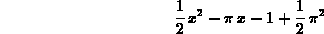
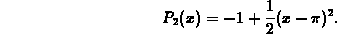
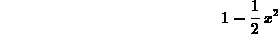
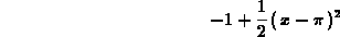
For example, using the formula in the theorem, we would write the
quadratic Taylor polynomial approximation to  with base
point
with base
point  as
as
The general formula may seem a little cumbersome at first, but you need to
become familiar with it. Note that x is the independent variable in
the formula, while a is a parameter that is either a constant or can
be treated as one. This means that things like  and
and  should be treated as constants.
Showing that the formula in the theorem satisfies the definition is
not difficult if you remember that x is the variable and a is a
parameter. Keeping this in mind, the first and second derivatives of
the formula in the theorem are 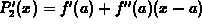 and
and
 .
Given the derivatives, showing that the formula in the theorem
satisfies the definition is simply a matter of substituting x=a.
.
Given the derivatives, showing that the formula in the theorem
satisfies the definition is simply a matter of substituting x=a.
The CalcP package has a command called Taylor that can be
used to generate quadratic Taylor polynomial approximations, as well
as the higher-order Taylor polynomial approximations that we'll study
later. (If you look at the help page for Taylor, you'll find out
that the third argument determines the order of the Taylor polynomial
generated. This argument is 2 in the examples because we are
generating the quadratic polynomials.) The Maple
commands given below provide examples of how to use this command in
generating, plotting, and manipulating quadratic Taylor polynomials.
The last example shows how to plot the absolute value of the error,
defined as  , of
a Taylor polynomial approximation.
, of
a Taylor polynomial approximation.
> with(CalcP):
> f(x);

> Taylor(f(x),x=Pi,2);

> Taylor(f(x),x=0,2);
> plot({f(x),Taylor(f(x),x=Pi,2)}, x=0..2*Pi);
> fquad := x-> Taylor(f(x),x=Pi,2) ;

> fquad(x);
> plot(abs(f(x)-fquad(x)),x=0..2*Pi);