cp ~bfarr/Probability_start.mws ~
You can copy the worksheet now, but you should read through the lab before you load it into Maple. Once you have read to the exercises, start up Maple, load the worksheet Probability_start.mws, and go through it carefully. Then you can start working on the exercises.
You may be more familiar with what are called discrete random
variables, for example the number of heads obtained in ten tosses of a
coin, which can only take a finite number of discrete values. In the
case of a discrete random variable, the probability of a single
outcome can be positive. For example, the probability that a single
flip of a coin produces tails is 50%. The situation is very different
when we consider a random variable like the number of miles a
tire can be driven before failure, which can take any value from
zero to something over ![]() miles. Since there are an infinite
number of possible outcomes, the probability that the tire
fails at exactly some number of miles, for example
miles. Since there are an infinite
number of possible outcomes, the probability that the tire
fails at exactly some number of miles, for example ![]() miles, is
zero. However, we would expect that the probability that the tire
would fail between
miles, is
zero. However, we would expect that the probability that the tire
would fail between ![]() miles and
miles and ![]() miles would not be
zero, but would be a positive number.
miles would not be
zero, but would be a positive number.
A random variable that can take on a continuous range of values is called a continuous random variable. There turn out to be lots of applications of continuous random variables in science, engineering, and business, so a lot of effort has gone into devising mathematical models. These mathematical models are all based on the following definition.
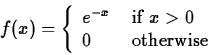
For example, consider the following function.
A lot of the effort involved in modeling a random process, that is, a
process whose outcome is a random variable, is in finding a suitable
probability density function. Over the years, lots of different
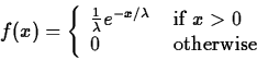
functions have been proposed and used. One thing that they all have in
common, though, is that they depend on parameters. For example, the
general exponential probability density function is defined as
The process of deciding what probability density function to use and
how to determine the parameters is very complicated and can involve
very sophisticated mathematics. However, in the simple approach we are
taking here, the problem of determining the parameter value(s) often
depends on quantities that can be determined experimentally, for
example by collecting data on tire failure. For our purposes, the two
most important quantities are the mean, ![]() and the standard
deviation
and the standard
deviation ![]() . The mean is defined by
. The mean is defined by
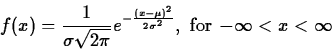
Probably the most important distribution is the normal distribution,
widely referred to as the bell-shaped curve. The probability density
function for a normal distribution with mean ![]() and standard
deviation
and standard
deviation ![]() is given by the following equation.
is given by the following equation.
In applications, one generally has to know in advance that the random variable you want to model folows a certain kind of distribution, at least approximately. How one would determine this is way beyond the scope of this course, so we won't really discuss it. On the other hand, once you know, for example, that your random variable has a normal distribution you only need the values of the mean and the standard deviation to be able to model it. The exponential distribution is even simpler, since it only has one parameter, and you only need to know the mean of your random variable to use this distribution to model it.
One thing to keep in mind when you are using the normal distribution
as a model is that calculations can involve values of your random
variable that don't make physical sense. For example, suppose that a
machining operation produces steel shafts whose diameters have
a normal distribution, with a mean of ![]() inches and a standard
deviation of
inches and a standard
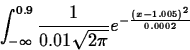
deviation of ![]() inch. If you were asked to compute the percentage of the
shafts in a certain production run that had diameters less than
inch. If you were asked to compute the percentage of the
shafts in a certain production run that had diameters less than ![]() inches you would use the following integral
inches you would use the following integral