In the previous lab, we introduced quadratic Taylor polynomial approximations. In this lab, we investigate higher-order Taylor polynomials.
The idea of the Taylor polynomial approximation of order n at
x=a, written  , to a smooth function
  is to require
that
is to require
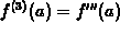
that  and
and  have the same value at x=a and,
furthermore, that their derivatives at x=a must match up to order
n. For example the Taylor polynomial of order three for
have the same value at x=a and,
furthermore, that their derivatives at x=a must match up to order
n. For example the Taylor polynomial of order three for  at
x=0 would have to satisfy the conditions
at
x=0 would have to satisfy the conditions
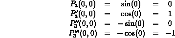
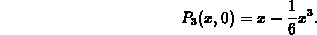
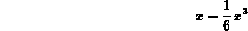
You should check for yourself that the cubic polynomial satisfying these four conditions is
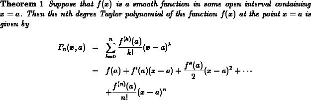
The general form of the Taylor polynomial approximation of order n
to  is given by the following
We will be seeing this formula a lot, so it
would be good for you to start memorizing it now! The notation
 is used in the definition to stand for the value of the
k-th derivative of f at x=a. That is,
is used in the definition to stand for the value of the
k-th derivative of f at x=a. That is, 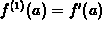 ,
,
 , and so on. By convention,
  . Note that a is fixed and so the derivatives
  are
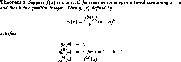
just numbers. The following easier theorem should help you to see
where the formula comes from.
are
just numbers. The following easier theorem should help you to see
where the formula comes from.
Maple has a command called taylor to generate these Taylor polynomial expansions, but the form it produces is not the most convenient, so two commands have been written as part of the CalcP package, which should be loaded with the following command.
> with(CalcP):
The two procedures are called Taylor and TayPlot. The
syntax for Taylor is
Taylor(f,x=a, n);,
where n is the order, f is an expression or a procedure, and a
is the base
point. The following examples should make the use of this procedure
clear. There is also help available with the command ?Taylor.
> Taylor(sin(x),x=0,3);
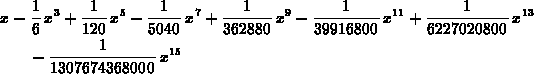
> Taylor(sin(x),x=0,15);
> Taylor(sin(x),x=Pi/6,4);

> Taylor(exp(x),x=0,5);

The result of this command is a polynomial expression that can be plotted, differentiated, etc.
It seems intuitive that the larger n is, the better the Taylor
polynomial will approximate  . To help you investigate this, a
procedure TayPlot has been written which plots
. To help you investigate this, a
procedure TayPlot has been written which plots  and a set of
Taylor polynomials simultaneously. The syntax for this command is
and a set of
Taylor polynomials simultaneously. The syntax for this command is
TayPlot(f,x=a,{n1,n2,n3, ...},x=b..d,ops);,
where f and x=a are as above, x=b..d is the usual x plot
range specifier, and ops are (optional) options that TayPlot
passes to the plot command. The set {n1,n2,n3, ...}
consists of integers corresponding to the Taylor polynomial
degrees desired. For example,
> TayPlot(sin(x),x=0,{2,3,5},x=-Pi..Pi);
> TayPlot(sin(x),x=0,{2,3,5},x=-Pi..Pi,y=-1.2..1.2);
are both valid calls of TayPlot. Both plot  and the
2nd, 3rd, and 5th order Taylor polynomial approximations. In the
second TayPlot command, the y range has been set to fit the
behavior of the
and the
2nd, 3rd, and 5th order Taylor polynomial approximations. In the
second TayPlot command, the y range has been set to fit the
behavior of the  function. You can plot
more than three Taylor polynomials if you want, of course. You can
also use a letter other than x for your independent variable. Help
for TayPlot is available with the ?TayPlot command.
function. You can plot
more than three Taylor polynomials if you want, of course. You can
also use a letter other than x for your independent variable. Help
for TayPlot is available with the ?TayPlot command.