Partial Sums

Note: The format for this lab is different from what you are used to. It consists of a series of exercises, with background material included in each exercise. You should read each question carefully before you try to answer it.

1.

Using the Integral Test We begin by considering the three series $$\sum^\infty_{n=1} \sqrt{n},\;\;\displaystyle\sum^\infty_{n=1} n^{-1/2}$$, and $$\sum^\infty_{n=1} n^{-3/2}$$. To gather information about these three series, let us first determine if they converge or diverge.

(a)

Write each of the three series as a p-series and determine if each converges or diverges using the integral test.

2.

Partial Sums

Having the information we found in problem (1a) regarding the convergence or divergence of each series, we will now look at some of the partial sums of these series to illustrate how important the integral test is in providing us with immediate insight into the convergence and divergence of a series.

(a)

Beginning with the first series, $$\sum^\infty_{n=1} \sqrt{n}$$ write out by hand the first five partial sums, $$\sum^m_{n=1} \sqrt{n}, m = 1,\ldots,5$$, of this series and use Maple to find the decimal values of each.

(b)

Based on the pattern you see developing, can you determine if this series converges or diverges? Why? As part of your discussion, use the shape of the graph of $f(x) = \sqrt{x}$ to aid in your reasoning.

(c)

Now write out the first five partial sums of the second and third series, $$\sum^\infty_{n=1} n^{-1/2}$$, and $$\sum^\infty_{n=1} n^{-3/2}$$ and again answer question (2b) for these series.

As you are now probably thinking, ``By just looking at the first few partial sums, one can not tell anything about the convergence or divergence of the series because in general a series will only reveal if it converges or diverges for large values of m''. And you are correct. So let us use Maple to look at the partial sums for larger values of m.

To look at partial sums in Maple we must first create a function that defines the sequence of partial sums. For example, let us consider $\{a_n\} = \{f(n)\}$, then the function that defines the m^th partial sum of the series $$\sum^\infty_{n=1} a_n$$ is:

Once we have defined this function, we can visually observe how the partial sums are changing by plotting the points (m, S_m) for $m = 1,2,3 \ldots$. Note that the x-coordinate indicates which partial sum we are considering and the y-coordinate is that partial sum. The syntax in Maple to define equation (1) is:

  > partial_sum:=m->sum(f(n),n=1..m);

This syntax defines the function partial_sum(m) as the sum of f(n) from 1 to m. To evaluate this function for various values of m, we use typical function syntax. For example, if we wanted the third partial sum of the series, we would type:

  > partial_sum(3);

Note that the partial_sum command assumes that you have defined a function f in Maple that satisfies f(n) = a_n. In the exercises below, you will be working with two series, so you will have to define one such function for each series. You will also have to define a separate command like partial_sum for each series.

To generate a sequence of partial sums beginning with the first one, we use the seq command in Maple:

  > seq(partial_sum(m),m=1..10);

This will give us a list of partial sums S_m of a series for $m = 1,2,3,\ldots,10$. To start with a partial sum other than the first, or to end with a partial sum different from the tenth, just adjust the arguments in the command.

Now to plot a sequence of the partial sums S_m for $m = 1,2,3,\ldots,b$ we type:

  > partial_sum_points:=[seq([m,partial_sum(m)],m=1..b)]:

  > plot(partial_sum_points,style=point);

The first command creates the set of points to be graphed and the second command graphs the points. Note the colon at the end of the first command, it is used to suppress the result, if a semi-colon was used instead, Maple would display the points that it created. Note also that the parameter b in the example stands for the highest partial sum you want to include in the plot.

(d)

Plot the first 20 partial sums of the series $$\sum^\infty_{n=1} n^{-1/2}$$ and $$\sum^\infty_{n=1} n^{-3/2}$$ on the same set of axes. (Remember for two plots on one set of axes you use {} to group the points as follows:

> plot({partial_sum_points1,partial_sum_points2}, style =
point);

where partial_sum_points1 and partial_sum_points2 are lists of points that have been previously defined.) From this plot are you able to determine if either sequence is converging or diverging? If yes, which one and why? To determine which plot belongs to which sequence it may be helpful to find the first few partial sums for each series. Label which graph belongs to which sequence of partial sums.

(e)

To explore this phenomenon further, try plotting the first 100 partial sums of these two series on one set of axes. Do these plots confirm your answer to (2d) or help you form an answer about the convergence or divergence of these series? Again label by hand which graph belongs to which sequence of partial sums.

In your answer to (2d) and (2e) you hopefully identified the lower sequence as the sequence of partial sums for the series $$\sum^\infty_{n=1} n^{-3/2}$$. But what about the other sequence of partial sums? Without the integral test, can you be sure that the series $$\sum^\infty_{n=1} n^{-1/2}$$, diverges from only looking at the graph? What if this series converged to a number larger than 20, then this would not be shown by our graph for the sequence of the first 100 partial sums of $$\sum^\infty_{n=1} n^{-1/2}$$. We could now look at the first 200 partial sums and so on hoping that eventually we would see the graph flatten out or rise sufficiently so that we could conclude that the sequence converged or diverged respectively, but that could take forever. And if we concluded that the sequence diverged, could we ever really be sure that it did not converge for some value of m larger than we considered? In reality that answer to this question is no, leading us to conclude that the convergence tests for series that we are learning in chapter 11 are crucial to know because they allow for speed and confidence when determining if a series converges or not.

(3)

Using Partial Sums to Create Approximations

In this part of the lab, we will examine how partial sums can be useful in creating approximations to functions. An example of this is Fourier series. A Fourier series is used to create an approximation to a periodic function by representing the function as a sum of sinusoids. This is helpful because while periodic functions have ``corners'', sinusoids are infinitely smooth functions, that is, they have derivatives of any order. Fourier series are most often used to aid in the analysis of mechanical or electrical systems.

The Fourier series

approximates the function shown below.

We will now examine a few of the partial sums of this sequence to see how the approximation improves as the number of terms included in the sum increases.

(a)

Enter the Fourier series F(m) into Maple.

(b)

Find the first, fourth, tenth, and hundredth partial sums of equation (2) and plot your results on different sets of axes. For these graphs, it is most straightforward to use the plot command as you have done in other labs. For example, if you defined the function fourier_series(m) to be the $m^{\mathrm{th}}$ partial sum of the Fourier series, then to plot the third partial sum you would type the following command.

  > plot(fourier_series(3),t=0..5);

The range of t values ($0 \leq t \leq 5$) is a good one to use in your plots. Describe your results.

(4)

Sphereflakes

Using Netscape (or some browser) look at the figure on the following web page:

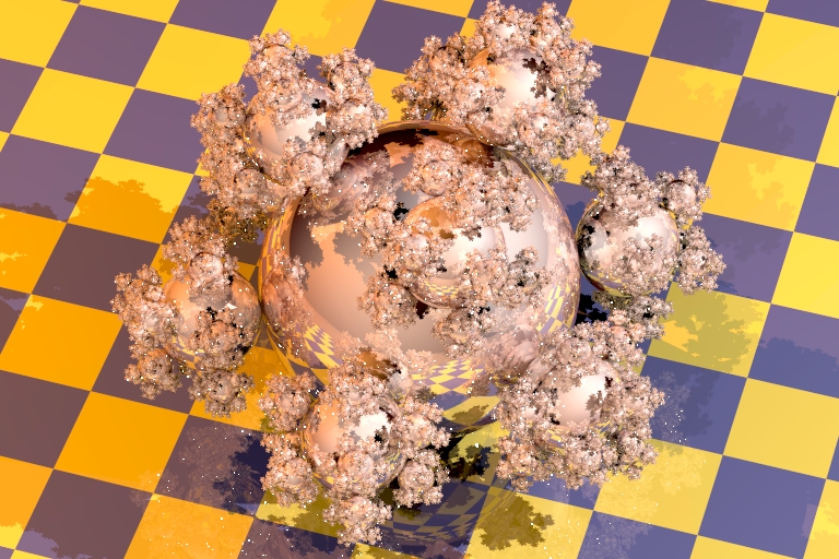
Sphereflake

This is a sphereflake. The radius of the largest sphere is 1. Attached to the largest sphere are 9 spheres of radius $$\frac{1}{3}$$. Attached to each of these nine spheres, are 9 more spheres of radius $$\frac{1}{9}$$, with this process continued indefinitely. Using series, prove that the sphereflake has an infinite surface area. Why does your answer seem visually impossible?