Taylor Polynomials and the Error

Maple Usage for Taylor Polynomials

Maple has a command called taylor that will generate Taylor polynomials. However, the form of its output is not convenient and so two commands which will better suit our purposes have been placed in the CalcP package. These are Taylor and TayPlot. Remember, that in order to use these two commands, you must first load the CalcP package as indicated below.

> with(CalcP):

If you are getting an error message with this command, you probably haven't copied a needed initialization file to your home directory. Look here to see how to do that.

To generate the Taylor polynomial P₃(x; 0) for sin(x), the syntax would be the following

> Taylor(sin(x), x=0, 3);

The Taylor polynomial P₄(x;

/6) for sin(x) would be produced by this command.

> Taylor(sin(x), x=Pi/6, 4);

For values of x sufficiently close to the base point x=a, the larger n gets, the better the Taylor polynomial P_n approximates the values of f.

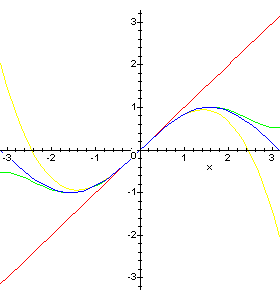
The TayPlot command will give you the graph of f(x) and the graphs of P_n(x; c) for a set of n values you select. That way you can see if the graph of P_n(x; c) becomes more like the graph of f(x) as larger values of n are used. To get a single plot which superimposes the graphs of P₁(x; 0), P₃(x; 0), and P₅(x; 0) on the graph of sin(x) over the interval from - to , you would use the following syntax.

> TayPlot(sin(x), x=0, {1,3,5}, x=-Pi..Pi);

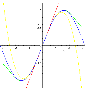
It is also possible to specify the y range for the plot as is done below.

> TayPlot(sin(x), x=0, {1,3,5}, x=-Pi..Pi, y=-1.2..1.2);

More than three Taylor polynomials may be plotted at a time. But, if too many are plotted, the plot will be too full to be useful.

Error

Let R_n(x; c) = f(x) - P_n(x; c). It can be instructional to graph |R_n(x; c)| on the interval under consideration. Designate the maximum of |R_n(x; c)| on the interval by E_n. The graphing can be accomplished in this way

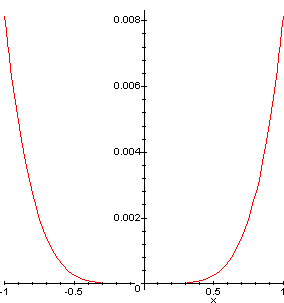
> plot(abs(sin(x)-Taylor(sin(x), x=0,3)), x=-1..1);

From the graph it can be seen that E₃ ~ 0.008.

Suppose you need to find n such that when P_n(x; 0) is used to approximate sin(x) you will have E_n < 0.005 on the interval [-1, 1]. Guess at n and make a try.

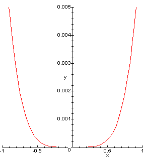
> plot(abs(sin(x)-Taylor(sin(x), x=0,3)), x=-1..1, y=0..0.005);

In looking at this plot you can see that the curve goes out of the region at the top of the window. This means that E₃ > 0.005. So, experiment a little more; use a larger value of n. Try again, using 5 instead of 3. Now the curve goes out the sides of the window. This says that E₅ < 0.005.