Many applications of calculus involve finding the maximum and minimum values of functions. For example, suppose that there is a network of electrical power generating stations, each with its own cost for producing power, with the cost per unit of power at each station changing with the amount of power it generates. An important problem for the network operators is to determine how much power each station should generate to minimize the total cost of generating a given amount of power.
In single-variable calculus, you found that one can locate candidates for local extreme values by finding points where the first derivative vanishes. For functions of two dimensions, the condition is that both first order partial derivatives must vanish at a local extreme value candidate point. Such a point is called a stationary point. It is also one of the three types of points called critical points. Note well that the condition does not say that a point where the partial derivatives vanish must be a local extreme point. Rather, it says that stationary points are candidates for local extrema. Just as was the case for functions of a single variable, there can be stationary points that are not extrema. For example, the saddle surface f(x,y)= x2 - y2 has a stationary point at the origin, but it is not a local extremum.
Finding and classifying the local extreme values of a function f requires several steps. Please refer to your text for the complete test. First, the partial derivatives must be computed. Then the stationary points must be solved for, which is not always a simple task. Next, one must check for the presence of singular points, i.e., points where the function is not differentiable. If any such points exist, they must be checked separately, probably by plotting the graph of the function. which might also be local extreme values. Finally, each critical point must be classified as a local maximum, local minimum, or neither.
In order to use the Maple commands for this lab you will need to load the plots package.
> with(plots):The following example is one that could be done by hand without too much work. First define the function.
> f:=(x,y)->x^2+2*y^2;Many times, plotting the function first helps you plan what to do next. From the plot below, we can tell that this function is minimized there.
> plot3d(f(x,y),x=-3..3,y=-3..3);A contour plot can also be useful for finding the approximate location of a critical point.
> contourplot(f(x,y),x=-3..3,y=-3..3);Finding the critical point is easy to do with the solve command. Given that the function is differentiable, one must find values of (x,y) where both first partial derivatives are zero:
> solve({diff(f(x,y),x)=0,diff(f(x,y),y)=0},{x,y});
The second partial test can be performed to check the conclusion from the plots.
This requires one to compute the discriminant
> subs({x=0,y=0},diff(f(x,y),x,x)*diff(f(x,y),y,y)-diff(f(x,y),x,y)^2);
Since the value we computed above is positive,
we must check the sign of the second partial derivative with respect to x.
> subs({x=0,y=0},diff(f(x,y),x,x));
It is positive, which verifies that we have a local minimum.
This next example shows output in Maple that you might run into and how to handle it. In this example the solve command uses the RootOf notation that may be unfamiliar to you.
> h:=(x,y)->(x^2+2*y)*(-x^2+y^2+1);Here we try the solve command. If you haven't seen the RootOf notation before, you may find it confusing. Essentially Maple uses this notation as a shorthand for multiple roots. The result below shows two families of solutions. The variable Z in a RootOf expression should be thought of as a placeholder.
> sol:=solve({diff(h(x,y),x)=0,diff(h(x,y),y)=0},{x,y});
The allvalues command can be used to expand a RootOf structure.
Here we pick out the first family of solutions,
which was x=0,y=RootOf( 1 + 32Z).
What this says is that x = 0 and y is any root
of the equation 1 + 3y2 = 0.
The allvalues command solves for the two roots.
Note that they are both complex and would be discarded,
since we only care about real critical points. Note also that we gave our solve command a label,
which made it easy to extract the first family of solutions.
  > allvalues(sol[1]);
  > allvalues(sol[2]);
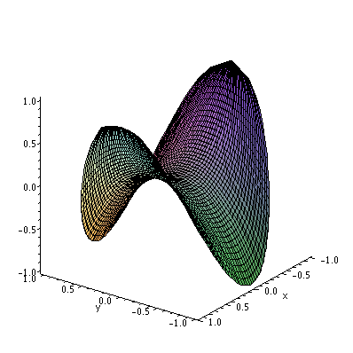
A contour plot seems to indicate that neither critical point is a local extrema.
> contourplot(h(x,y),x=-2..2,y=-2..2);Using the plot3d, it is pretty clear that both critical points are saddle points.
> plot3d(h(x,y),x=-2..2,y=-2..2);If we attempt to use the second partials test on this example, we get zero at both of the stationary points. (one of these is shown below.) Getting zero means that the test fails. In this case the plots are more useful.
> subs({x=sqrt(2),y=-1},diff(h(x,y),x,x)*diff(h(x,y),y,y)-diff(h(x,y),x,y)^2);
The basic theorem on the existence of global maximum and minimum values is the following.
If you are told to find the global extrema of h(x,y) from above with the domain -2 &le x &le 2 and -2 &le y &le 2 you need to check the stationary points and the boundaries which includes the two-dimensional functions on the edges as well as the corner points. Set the first derivative equal to zero along the four planar edges. You can do this in Maple by specifying the plane within the function itself. In the y = -2 plane the function is h(x,-2). Solve for the critical points.
  > a:=solve(diff(h(x,-2),x)=0,x);
  > evalf(a);
Notice that two of these critical points are outside the domain, leaving the critical point of (0, -2) and the two corner points (-2, -2) and (2, -2) on this edge of the domain. Remember with global extrema you are only concerned with the highest and lowest f-value. After you find all possible points within the domain and its boundary, substitute into the function to find the f-values.
Written by:
JDF
(E-Mail: bach@wpi.edu)
Last Updated: Monday, 25 September 2006
Copyright 2006, William F. Farr, Joseph D. Fehribach