Subsections

• Purpose
• Getting Started
• Background
  • Different parametric descriptions of a curve in the plane
  
  
• Exercises

Visualizing parametric curves in the plane

Purpose

The purpose of this lab is to give you practice with parametrizing curves in the plane and in visualizing parametric curves as representing motion.

Getting Started

To assist you, there is a worksheet associated with this lab that contains examples and even solutions to some of the exercises. You can copy that worksheet to your home directory with the following command, which must be run in a terminal window, not in Maple.

cp ~bfarr/Parametric_start.mws ~

You can copy the worksheet now, but you should read through the lab before you load it into Maple. Once you have read to the exercises, start up Maple, load the worksheet Parametric_start.mws, and go through it carefully. Then you can start working on the exercises

Background

A parametric curve in the plane can be defined as an ordered pair, $(f(t), g(t))$, of functions, with $f(t)$ representing the $x$ coordinate and $g(t)$ the $y$ coordinate. Parametric curves arise naturally as the solutions of differential equations and often represent the motion of a particle or a mechanical system. They also often arise in studying oscillations in electrical circuits.

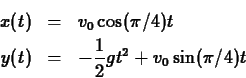
For example, neglecting air resistance, the position of a projectile fired from the origin at an initial speed of $v_0$ and angle of inclination $\pi/4$ is given by the parametric equations

$$\begin{eqnarray*} x(t) & = & v_0 \cos(\pi/4) t \\ y(t) & = & -\frac{1}{2} g t^2 + v_0 \sin(\pi/4) t \end{eqnarray*}$$

where $t$ is time and $g$ is the acceleration due to gravity.

Graphically, a parametric curve can be represented several ways. One simple way is to plot the component functions, $f(t)$ and $g(t)$, individually versus the independent variable $t$. Another way is to plot the set of points $\{(f(t),g(t)): t \mbox{ in } {\bf R}\}$. This gives you the curve along which the particle moves, but information on how it moves has been lost. On the other hand, plotting the component functions individually makes it hard to see how the particle is actually moving.

To help you to visualize parametric curves as representing motion, a Maple routine called ParamPlot has been written. It uses the Maple animate command to actually show the particle moving along its trajectory. You actually used this command last term for the lab on polar coordinates. Examples are in the Getting Started worksheet.

Different parametric descriptions of a curve in the plane

Given a curve defined by the graph of a function $y=h(x)$, there are an infinite number of ways of representing this curve parametrically, corresponding to different motions on the curve. About the simplest way of parametrizing $y=h(x)$ is with the pair $(t,h(t))$, which traverses the curve from left to right as $t$ increases. One can reverse the direction of motion by changing to the parametrization $(-t,h(t))$.

By restricting $t$ to an interval $[a,b]$, you can get a parametric description of a portion of the curve. For example, the right half of the parabola $y=x^2$ would result from $(t,t^2)$ for $t \geq 0$.

More complicated parametrizations of $y=h(x)$ can be obtained with parametric curves of the form $(f(t),h(f(t)))$. By choosing $f(t)$ appropriately, for example, you can make the particle stop and turn back on the curve. For example, suppose that the curve to be parametrized is the graph of the function $y=2x$. The following examples give three different parametrizations of parts of this curve.

$$x(t) = \sin(t) \; \; y(t) = 2 \sin(t) \; \; 0 \leq t \leq 4 \pi$$

$$x(t) = t-1 \; \; y(t) = 2t-2 \; \; 0 \leq t 2$$

$$x(t) = (1-t)^2 \; \; y(t) = 2 (1-t)^2 \; \; 0 \leq t \leq3$$

Exercises

1. The cycloid is a famous example of a parametric curve having several important applications. Use the ParamPlot command to animate the cycloid $x(t) = t-\cos(t)$, $y(t) = 1-\sin(t)$ over the interval $0 \leq t \leq 6 \pi$ and then use the plot command to generate a printable plot of this cycloid over the same interval.

2. The family of parametric curves
   
   $$( \cos(n t), \sin(m t)), \mbox{ for $0 \leq t \leq 2 \pi$},$$
   
   
   where $n$ and $m$ are positive integers, is an example of what is called a Lissajous figure. Use ParamPlot to plot the two cases $n=1,m=2$ and $n=1,m=3$ and describe what you see. Include printable plots of each curve in your printout.

3. The last example, concerning the straight line $y=2x$, provided three different parametrizations. Match the parametrizations with the descriptions below. Justify your choices.
   1. Starts at the point $(1,2)$. Moves to the left initially, but reverses direction once.
   2. Starts at the origin, then oscillates between the points $(1,2)$ and $(-1,-2)$.
   3. Starts at the point $(-1,-2)$ and then moves to the right along the line.

4. Given the function $y=x^3-x$, find a function $f(t)$ that makes the parametric description $(f(t), f(t)^3-f(t))$ do the following. Make sure that you explain your choices.
   1. Goes through the origin at $t=0$ and traverses the curve from right to left as $t$ increases.
   2. Goes through the origin at $t=0$ and oscillates between the points $(1,0)$ and $(-1,0)$.