Next: About this document ...
Up: lab_template
Previous: lab_template
Subsections
The purpose of this lab is to introduce you to curve computations
using Maple for parametric curves and vector-valued functions in three
dimensions.
To assist you, there is a worksheet associated with this lab that
contains examples. You can
copy that worksheet to your home directory with the following command,
which must be run in a terminal window, not in Maple.
cp ~bfarr/Curves3D_start.mws ~
You can copy the worksheet now, but you should read through the lab
before you load it into Maple. Once you have read to the exercises,
start up Maple, load
the worksheet Curves3D_start.mws, and go through it
carefully. Then you can start working on the exercises
A parametric curve in three dimensions is a triple of functions
 ,
,  ,
,  for
for  in some interval
  .
A vector-valued function in
three dimensions is a function
.
A vector-valued function in
three dimensions is a function  that associates a vector in
the plane with
each value of in its domain. Such a vector valued function can
always be
written in component form as follows,
that associates a vector in
the plane with
each value of in its domain. Such a vector valued function can
always be
written in component form as follows,
where  ,
,  , and
, and  are functions defined on some interval . From our
definition of a parametric curve, it should be clear that you can
always associate a
parametric curve with a vector-valued function by just considering the
curve traced out by the head of the vector. However, there are
lots of situations where a vector-valued function is more
appropriate. We will focus on
the case of motion of a particle in three dimensions. That is, we have a
vector-valued function that gives the position at time
of a moving point
are functions defined on some interval . From our
definition of a parametric curve, it should be clear that you can
always associate a
parametric curve with a vector-valued function by just considering the
curve traced out by the head of the vector. However, there are
lots of situations where a vector-valued function is more
appropriate. We will focus on
the case of motion of a particle in three dimensions. That is, we have a
vector-valued function that gives the position at time
of a moving point  . The velocity of this point is
given by the derivative
. The velocity of this point is
given by the derivative
 and the acceleration is given
by the second derivative,
and the acceleration is given
by the second derivative,
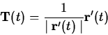
 . If the velocity,
, is never zero, then we can define the unit tangent
vector
. If the velocity,
, is never zero, then we can define the unit tangent
vector  and the curvature
  the same way we
did in two dimensions by
the same way we
did in two dimensions by
and
If the curvature is never zero for a particular curve, then we can
define another intrinsic property of curve, the unit normal vector
 by the following equation.
It can be shown that at each point on the curve the vector defined
by this equation is a unit vector that is always perpendicular to the
tangent vector  at that point. Furthermore, the unit normal vector
always points in the direction of the centripetal
acceleration required to keep a particle moving on the curve. One way
to see this is to compute the acceleration by differentiating both
sides of the equation
at that point. Furthermore, the unit normal vector
always points in the direction of the centripetal
acceleration required to keep a particle moving on the curve. One way
to see this is to compute the acceleration by differentiating both
sides of the equation
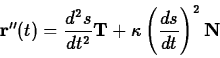
Using the chain rule and the definition of the
curvature and the normal vector one obtains the following important
equation.
To see why this equation is useful, recall that  is the
speed, so
is the
speed, so  is the rate of change of the speed.
That is, this term measures whether the particle is speeding up or
slowing down. Because this component of the
acceleration is in the direction of the tangent vector it is often
called the tangential acceleration, denoted by the symbol
is the rate of change of the speed.
That is, this term measures whether the particle is speeding up or
slowing down. Because this component of the
acceleration is in the direction of the tangent vector it is often
called the tangential acceleration, denoted by the symbol  . The
component of the acceleration in the direction of the normal vector is
called the normal acceleration, denoted
. The
component of the acceleration in the direction of the normal vector is
called the normal acceleration, denoted  . In the case of motion
on a circular path, the curvature is the reciprocal of the radius, so
this term should be easily recognizable as the centripetal
acceleration.
. In the case of motion
on a circular path, the curvature is the reciprocal of the radius, so
this term should be easily recognizable as the centripetal
acceleration.
Computing these quantities is generally not an
easy task. The Getting started worksheet for this lab
describes commands from the CalcP package that simplify these
calculations and provides examples for you to work from.
- Consider the circular helix
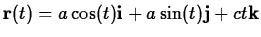 . Plot the graphs
for the following sets of values of
. Plot the graphs
for the following sets of values of  and
and  using the
VPlot command. You should also look at animations of the
plots by using the ParamPlot3D command, though they won't
appear in your printout.
using the
VPlot command. You should also look at animations of the
plots by using the ParamPlot3D command, though they won't
appear in your printout.
 ,
,  for
for
 .
.
- ,
 for
.
for
.
 , for
.
, for
.
Give a brief explanation of how the values of and affect the
graph.
- Consider again the circular helix
. Compute the speed
and the curvature as functions of the parameters and and
relate your results to your findings from the first exercise.
- Consider the function
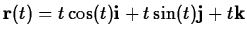 that appeared as one
of the examples.
that appeared as one
of the examples.
- Compute the curvature, and plot it for
.
- Compute the normal acceleration, and plot it for
.
- Can you explain why the normal acceleration is increasing, even
though the curvature is decreasing?
Next: About this document ...
Up: lab_template
Previous: lab_template
William W. Farr
2003-11-10