Next: About this document ...
Up: lab_template
Previous: lab_template
Subsections
The purpose of this lab is to acquaint you with using Maple to compute
partial derivatives, directional derivatives, and the gradient.
To assist you, there is a worksheet associated with this lab that
contains examples. You can
copy that worksheet to your home directory with the following command,
which must be run in a terminal window, not in Maple.
cp ~bfarr/Pardiff_start.mws ~
You can copy the worksheet now, but you should read through the lab
before you load it into Maple. Once you have read to the exercises,
start up Maple, load
the worksheet Pardiff_start.mws, and go through it
carefully. Then you can start working on the exercises.
For a function  of a single real variable, the derivative
 gives information on whether the graph of
  is increasing or
decreasing. Finding where the derivative is zero was important in
finding extreme values. For a function
is increasing or
decreasing. Finding where the derivative is zero was important in
finding extreme values. For a function  of two (or more)
variables, the situation is more complicated.
of two (or more)
variables, the situation is more complicated.
A differentiable function, , of two variables has two partial
derivatives:
 and
and
 . As you have learned in class, computing partial derivatives is
very much like computing regular derivatives. The main difference is
that when you are computing
, you must treat
the variable
. As you have learned in class, computing partial derivatives is
very much like computing regular derivatives. The main difference is
that when you are computing
, you must treat
the variable  as if it was a constant and vice-versa when computing
.
as if it was a constant and vice-versa when computing
.
The Maple commands for computing partial derivatives are D
and diff. The Getting Started worksheet has examples
of how to use these commands to compute partial derivatives.
The partial derivatives
and
of  can be thought of as the rate of change of in
the direction parallel to the
can be thought of as the rate of change of in
the direction parallel to the  and axes, respectively. The
directional derivative
and axes, respectively. The
directional derivative
 , where
 is a unit vector, is the rate of change of in the
direction . There are several different ways that the
directional derivative can be computed. The method most often used
for hand calculation relies on the gradient, which will be described
below. It is also possible to simply use the definition
is a unit vector, is the rate of change of in the
direction . There are several different ways that the
directional derivative can be computed. The method most often used
for hand calculation relies on the gradient, which will be described
below. It is also possible to simply use the definition
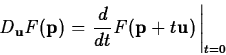
to compute the directional derivative. However, the following
computation, based on the definition, is often simpler to use.
One way to think about this that can be helpful in understanding
directional derivatives is to realize that
 is
a straight line in the
is
a straight line in the  plane. The plane perpendicular to the
plane that contains this straight line intersects the surface
plane. The plane perpendicular to the
plane that contains this straight line intersects the surface  in a curve whose
  coordinate is
 . The derivative of
at
. The derivative of
at  is the rate of change of at
the point
is the rate of change of at
the point  moving in the direction .
Maple doesn't have a simple command for computing directional
derivatives. There is a command in the tensor package that
can be used, but it is a little confusing unless you know something
about tensors. Fortunately, the method described above and the method
using the gradient described below are both easy to implement in
Maple. Examples are given in the Getting Started worksheet.
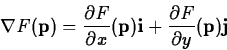
The gradient of , written  , is most easily computed as
As described in the text, the gradient has several important
properties, including the following.
Maple has a fairly simple command grad in the linalg
package (which we used for curve computations). Examples of computing
gradients, using the gradient to compute directional derivatives, and
plotting the gradient field are all in the Getting Started
worksheet.
- Consider the following function from the previous lab.
First, plot the graph of this function over the domain
 and
and
 using the plot3d
command. Then use the
contourplot command to generate a contour plot of
using the plot3d
command. Then use the
contourplot command to generate a contour plot of  over
the same domain.
over
the same domain.
- Compute the two first order partial derivatives of the function
in the first exercise.
You may use either the D or diff commands. Then evaluate
them at the point
 ,
,  and explain the values you get in
terms of the plots in the first exercise.
and explain the values you get in
terms of the plots in the first exercise.
- Consider again the function from the first exercise. Using
either method from the Getting Started compute the
directional derivative of at the point ,
 in the
three directions below. You may want to put an evalf command
on the outside to get numerical values.
in the
three directions below. You may want to put an evalf command
on the outside to get numerical values.
-
-

-

- Using the method from the Getting Started worksheet,
plot the gradient field and the contours of on the same plot. Use
the same domain of
and
. Can you
use this plot to explain the values for the directional derivatives
you obtained in the previous exercises? By explaining the values, I
only mean can you explain why the values were positive, negative, or
zero in terms of the contours and the gradient field?
Next: About this document ...
Up: lab_template
Previous: lab_template
William W. Farr
2003-11-30