Next: About this document ...
Up: lab_template
Previous: lab_template
Subsections
The purpose of this lab is to introduce you to curve computations
using Maple for parametric curves and vector-valued functions in three
dimensions.
To assist you, there is a worksheet associated with this lab that
contains examples. You can
copy that worksheet to your home directory with the following command,
which must be run in a terminal window, not in Maple.
cp ~bfarr/Curves3D_start.mws ~
You can copy the worksheet now, but you should read through the lab
before you load it into Maple. Once you have read to the exercises,
start up Maple, load
the worksheet Curves3D_start.mws, and go through it
carefully. Then you can start working on the exercises
A parametric curve in three dimensions is a triple of functions
 ,
,  ,
,  for
for  in some interval
  .
A vector-valued function in
three dimensions is a function
.
A vector-valued function in
three dimensions is a function  that associates a vector in
the plane with
each value of in its domain. Such a vector valued function can
always be
written in component form as follows,
that associates a vector in
the plane with
each value of in its domain. Such a vector valued function can
always be
written in component form as follows,
where  ,
,  , and
, and  are functions defined on some interval . From our
definition of a parametric curve, it should be clear that you can
always associate a
parametric curve with a vector-valued function by just considering the
curve traced out by the head of the vector. However, there are
lots of situations where a vector-valued function is more
appropriate. We will focus on
the case of motion of a particle in three dimensions. That is, we have a
vector-valued function that gives the position at time
of a moving point
are functions defined on some interval . From our
definition of a parametric curve, it should be clear that you can
always associate a
parametric curve with a vector-valued function by just considering the
curve traced out by the head of the vector. However, there are
lots of situations where a vector-valued function is more
appropriate. We will focus on
the case of motion of a particle in three dimensions. That is, we have a
vector-valued function that gives the position at time
of a moving point  . The velocity of this point is
given by the derivative
. The velocity of this point is
given by the derivative
 and the acceleration is given
by the second derivative,
and the acceleration is given
by the second derivative,
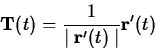
 . If the velocity,
, is never zero, then we can define the unit tangent
vector
. If the velocity,
, is never zero, then we can define the unit tangent
vector  and the curvature
  the same way we
did in two dimensions by
the same way we
did in two dimensions by
and
If the curvature is never zero for a particular curve, then we can
define another intrinsic property of curve, the unit normal vector
 by the following equation.
It can be shown that at each point on the curve the vector defined
by this equation is a unit vector that is always perpendicular to the
tangent vector  at that point. Furthermore, the unit normal vector
always points in the direction of the centripetal
acceleration required to keep a particle moving on the curve. One way
to see this is to compute the acceleration by differentiating both
sides of the equation
at that point. Furthermore, the unit normal vector
always points in the direction of the centripetal
acceleration required to keep a particle moving on the curve. One way
to see this is to compute the acceleration by differentiating both
sides of the equation
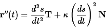
Using the chain rule and the definition of the
curvature and the normal vector one obtains the following important
equation.
To see why this equation is useful, recall that  is the
speed, so
is the
speed, so  is the rate of change of the speed.
That is, this term measures whether the particle is speeding up or
slowing down. Because this component of the
acceleration is in the direction of the tangent vector it is often
called the tangential acceleration, denoted by the symbol
is the rate of change of the speed.
That is, this term measures whether the particle is speeding up or
slowing down. Because this component of the
acceleration is in the direction of the tangent vector it is often
called the tangential acceleration, denoted by the symbol  . The
component of the acceleration in the direction of the normal vector is
called the normal acceleration, denoted
. The
component of the acceleration in the direction of the normal vector is
called the normal acceleration, denoted  . In the case of motion
on a circular path, the curvature is the reciprocal of the radius, so
this term should be easily recognizable as the centripetal
acceleration.
. In the case of motion
on a circular path, the curvature is the reciprocal of the radius, so
this term should be easily recognizable as the centripetal
acceleration.
Computing these quantities is generally not an
easy task. The Getting started worksheet for this lab
describes commands from the CalcP package that simplify these
calculations and provides examples for you to work from.
- As described in the text, a curve of the form
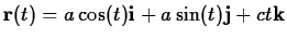 is called a circular
helix. It has the properties that the speed, curvature and normal and
tangential acceleration are all constant. Consider the vector-valued
function
is called a circular
helix. It has the properties that the speed, curvature and normal and
tangential acceleration are all constant. Consider the vector-valued
function
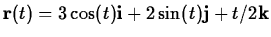 .
.
- Plot the graph of this function for
 . Explain why the graph might be called an elliptical helix. (Note
- the plot you get might make it look like a circular helix, that is
one whose projection in the
. Explain why the graph might be called an elliptical helix. (Note
- the plot you get might make it look like a circular helix, that is
one whose projection in the  plane is a circle, because of the
way Maple will scale the axes. The best way to overcome this is to
use the optional argument view. For example, try adding
plane is a circle, because of the
way Maple will scale the axes. The best way to overcome this is to
use the optional argument view. For example, try adding
view=[-3..3,-3..3,0..2*Pi]
to your VPlot command.)
- Plot the speed for
 . Is it constant?
- Plot the curvature for
. Is it constant?
- In the old days, students at WPI used to do projects in calculus
as well as labs. One such project called for students to design a loop for a
roller coaster. A group from the class of `95 came up with the
following design, which they called the ``Vomit Comet''.
Here is the position in units of meters of the car on the loop
and is the time in seconds.
- Plot the position for
 . The best way to view
the loop is probably looking in along the
. The best way to view
the loop is probably looking in along the  axis. How high
(approximately) is the top of the loop, in meters?
axis. How high
(approximately) is the top of the loop, in meters?
- Find the speed of the car and convert it to units of miles per
hour ( 1 meter per second is about 2.24 miles per hour). Does it seem
reasonable for a roller coaster?
- Plot the curvature of the loop for
.
- What is the radius of curvature of the loop at
 ? At
? At  ?
?
- Plot the normal acceleration of the loop for
. To put it in perspective, you might want to plot the normal
acceleration divided by
 , the acceleration due to gravity in
units of meters per second squared.
, the acceleration due to gravity in
units of meters per second squared.
- Based on your results, do you think the loop lives up to its name?
Next: About this document ...
Up: lab_template
Previous: lab_template
William W. Farr
2003-01-20