Next: About this document ...
Up: lab_template
Previous: lab_template
Subsections
The purpose of this lab is to acquaint you with techniques for finding
and classifying local and global extreme values of functions of two
variables.
To assist you, there is a worksheet associated with this lab that
contains examples. You can
copy that worksheet to your home directory with the following command,
which must be run in a terminal window, not in Maple.
cp ~bfarr/Extrema2D_start.mws ~
You can copy the worksheet now, but you should read through the lab
before you load it into Maple. Once you have read to the exercises,
start up Maple, load
the worksheet Extrema2D_start.mws, and go through it
carefully. Then you can start working on the exercises.
Many applications of calculus involve finding the maximum and minimum
values of functions. For example, suppose that there is a network of
electrical power generating stations, each with its own cost for
producing power, with the cost per unit of power at each station
changing with the amount of power it generates. An important problem
for the network operators
is to determine how much power each station should generate to
minimize the total cost of generating a given amount of power.
A crucial first step in solving such problems is being able to find
and classify local extreme values of a function. What we mean by a
function  having a local extreme value at a point
  is
that for values of
is
that for values of  near ,
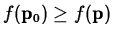 for a local maximum and
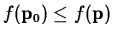 for a local minimum.
In single-variable
calculus, we found that we could locate candidates for local extreme
values by finding points where the first derivative vanishes. For
functions of two dimensions, the condition is that both first order
partial derivatives must vanish at a local extreme value candidate
point. Such a point is called a stationary point. It is also one of
the three types of points called critical points.
Note carefully that the condition does not say that a point where the partial
derivatives vanish must be a local extreme point. Rather, it says that
stationary points are candidates for local extrema. Just as was the case
for functions of a single variable, there can be stationary points that
are not extrema. For example, the saddle surface
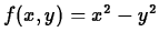 has a stationary point at the origin, but it is not a local extremum.
Finding and classifying the local extreme values of a function
 requires several steps. First, the partial derivatives must
be computed. Then the stationary points must be solved for, which is not
always a simple task. Next, one must check for the presence of
singular points, which might also be local extreme
values. Finally, each
critical point must be classified
as a local maximum, local minimum, or neither. The examples in the
Getting Started worksheet
are intended to help you learn how to use Maple to simplify these tasks.
requires several steps. First, the partial derivatives must
be computed. Then the stationary points must be solved for, which is not
always a simple task. Next, one must check for the presence of
singular points, which might also be local extreme
values. Finally, each
critical point must be classified
as a local maximum, local minimum, or neither. The examples in the
Getting Started worksheet
are intended to help you learn how to use Maple to simplify these tasks.
In one-dimensional calculus, the absolute or global extreme values of
a function occur either at a point where the derivative is zero, a
boundary point, or where the derivative fails to exist. The situation
for a function of two variables is very similar, but the problem is
much more difficult because the boundary now consists of curves
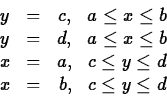
instead of just endpoints of intervals. For example, suppose that we
wanted to find the global extreme values of a function on the
rectangle
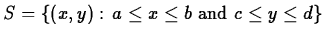 . The boundary of this rectangle consists of the four line
segments given below.
. The boundary of this rectangle consists of the four line
segments given below.
The basic theorem on the existence of global maximum and minimum values is
the following.
Theorem 1
Suppose
is continuous on a closed, bounded set

, then
attains its absolute
maximum value at some point

in
and absolute minimum value at
some point

in
.
This theorem only says that the extrema exist, but doesn't help at all
in finding them. However, we know that the global extrema occur either
at local extrema, on the boundary of the region, or at points where
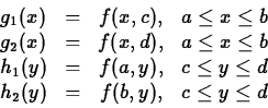
one or the other partial derivative fails to exist. For example, to
find the extreme values of a
function on the rectangle given above, you would first have to
find the interior critical points and then find the extreme values for
the four one-dimensional functions
- Find and classify the stationary points for the following
function.
- Consider the function
Find the absolute extrema of this function on the
rectangle
 ,
,
 .
.
- What is the maximum possible volume of a rectangular box
inscribed in a hemisphere of radius
 ? You may assume that one
face of the box lies in the planar base of the hemisphere.
? You may assume that one
face of the box lies in the planar base of the hemisphere.
Next: About this document ...
Up: lab_template
Previous: lab_template
William W. Farr
2004-02-13