Next: About this document ...
Up: lab_template
Previous: lab_template
Subsections
The purpose of this lab is to introduce you to curve computations
using Maple for parametric curves and vector-valued functions in the
plane.
To assist you, there is a worksheet associated with this lab that
contains examples and even solutions to some of the exercises. You can
copy that worksheet to your home directory with the following command,
which must be run in a terminal window, not in Maple.
cp ~bfarr/Curves2D_start.mws ~
You can copy the worksheet now, but you should read through the lab
before you load it into Maple. Once you have read to the exercises,
start up Maple, load
the worksheet Vec2D_start.mws, and go through it
carefully. Then you can start working on the exercises.
By parametric curve in the plane, we mean a pair of equations  and
and  for
for  in some interval
  . A vector-valued function in
the plane is a function
. A vector-valued function in
the plane is a function  that associates a vector in
the plane with
each value of in its domain. Such a vector valued function can
always be
written in component form as follows,
that associates a vector in
the plane with
each value of in its domain. Such a vector valued function can
always be
written in component form as follows,
where  and
and  are functions defined on some interval . From our
definition of a parametric curve, it should be clear that you can
always associate a
parametric curve with a vector-valued function by just considering the
curve traced out by the head of the vector.
are functions defined on some interval . From our
definition of a parametric curve, it should be clear that you can
always associate a
parametric curve with a vector-valued function by just considering the
curve traced out by the head of the vector.
For this lab, we will assume that we have a
vector-valued function that gives the position at time
of a moving point  in the plane. The velocity of this point is
given by the derivative
in the plane. The velocity of this point is
given by the derivative
 and the acceleration is given
by the second derivative,
and the acceleration is given
by the second derivative,
 .
In many applications of
curvilinear motion, we need to know the magnitude of the velocity, or
the speed. This is easy to compute - just take the magnitude
.
In many applications of
curvilinear motion, we need to know the magnitude of the velocity, or
the speed. This is easy to compute - just take the magnitude
 . If you think of the speed as the rate of change
of distance along the curve, and recall that arc length is distance
measured along the curve, then you have the following interpretation
of the speed
. If you think of the speed as the rate of change
of distance along the curve, and recall that arc length is distance
measured along the curve, then you have the following interpretation
of the speed
where  is arc length.
If the speed is not zero for any value of in the interval ,
then it is possible to define a unit vector,  that is
tangent to the curve as follows.
that is
tangent to the curve as follows.
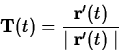
Using this definition, you can write the velocity in the following form.
This is not the most useful form for calculating the velocity, but it
does lead to a useful way of thinking about the acceleration
experience by a particle moving in a curvilinear path.
If the path is a straight line, acceleration depends only on
whether the particle is speeding up or slowing down. In a curve, however,
there is an additional acceleration, called the centripetal
acceleration, that is needed to keep the particle moving on the curve. The
magnitude of this acceleration depends on the speed of the car and how
much the path is curving. It turns out that you can quantify this
with an intrinsic property of the curve called
the curvature, usually denoted  , defined by the following
equation.
, defined by the following
equation.
That is, the curvature is the magnitude of the rate of change of the
tangent vector  with respect to arc length. For example,
the curvature of a straight line is zero and it can be shown that the
curvature of a circle of radius
with respect to arc length. For example,
the curvature of a straight line is zero and it can be shown that the
curvature of a circle of radius  is the same for every point on the
circle and is given by
is the same for every point on the
circle and is given by  .
.
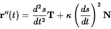
If the curvature is never zero for a particular curve, then we can
define another intrinsic property of curve, the unit normal vector
 by the following equation.
It can be shown that at each point on the curve the vector defined
by this equation is a unit vector that is always perpendicular to the
tangent vector  at that point. Furthermore, the unit normal vector
always points in the direction of the centripetal
acceleration required to keep a particle moving on the curve. In your
text, the following important relation is derived.
at that point. Furthermore, the unit normal vector
always points in the direction of the centripetal
acceleration required to keep a particle moving on the curve. In your
text, the following important relation is derived.
To see why this equation is useful, recall that  is the
speed, so
is the
speed, so  is the rate of change of the speed.
That is, this term measures whether the particle is speeding up or
slowing down. Because this component of the
acceleration is in the direction of the tangent vector it is often
called the tangential acceleration, denoted by the symbol
is the rate of change of the speed.
That is, this term measures whether the particle is speeding up or
slowing down. Because this component of the
acceleration is in the direction of the tangent vector it is often
called the tangential acceleration, denoted by the symbol  . The
component of the acceleration in the direction of the normal vector is
called the normal acceleration, denoted
. The
component of the acceleration in the direction of the normal vector is
called the normal acceleration, denoted  . In the case of motion
on a circular path, the curvature is the reciprocal of the radius, so
this term should be easily recognizable as the centripetal
acceleration for uniform circular motion.
. In the case of motion
on a circular path, the curvature is the reciprocal of the radius, so
this term should be easily recognizable as the centripetal
acceleration for uniform circular motion.
Computing these quantities is generally not an
easy task. The Getting started worksheet for this lab
describes commands from the CalcP package that simplify these
calculations and provides examples for you to work from.
- Consider the parametric curve
 ,
,  . Plot
the graph of this curve for
. Plot
the graph of this curve for
 . Identify the points
for
. Identify the points
for  ,
,  , and
, and  on your graph. Indicate the motion
on the curve as increases. This is probably best done by hand on
the printed copy.
on your graph. Indicate the motion
on the curve as increases. This is probably best done by hand on
the printed copy.
- For each of the following parametric curves, plot the graph and
locate the point on your graph that corresponds to
 .
.
-
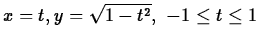
-
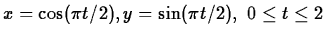
Explain why the graph is the same in each case, even though the
parametrizations are different.
- For following vector function, compute the unit
tangent vector , the unit normal vector
 , the curvature
  , and the normal and
tangential accelerations at the indicated value of . Include a plot
of the curve for the given interval in your worksheet.
, and the normal and
tangential accelerations at the indicated value of . Include a plot
of the curve for the given interval in your worksheet.
Compute ,
, , , and at 
Next: About this document ...
Up: lab_template
Previous: lab_template
William W. Farr
2004-01-16