Subsections

• Purpose
• Getting Started
• Background
  • Least Squares
  
  
• Exercises

MA 1024: The Extrema Test and the Least Squares Method of Approximation

Purpose

The purpose of this lab is to acquaint you with techniques for finding and classifying local and global extreme values of functions of two variables.

Getting Started

To assist you, there is a worksheet associated with this lab that contains examples. You can copy that worksheet to your home directory with the following command, which must be run in a terminal window, like teraterm, not in Maple.

cp /math/calclab/MA1024/least_squares.mws My_Documents

You can copy the worksheet now, but you should read through the lab before you load it into Maple. Once you have read to the exercises, start up Maple, load the worksheet least_squares.mws, and go through it carefully. Then you can start working on the exercises.

Background

Many applications of calculus involve finding the maximum and minimum values of functions. For example, suppose that there is a network of electrical power generating stations, each with its own cost for producing power, with the cost per unit of power at each station changing with the amount of power it generates. An important problem for the network operators is to determine how much power each station should generate to minimize the total cost of generating a given amount of power.

A crucial first step in solving such problems is being able to find and classify local extreme values of a function. What we mean by a function $f$ having a local extreme value at a point $\mathbf{p}_0$ is that for values of $\mathbf{p}$ near $\mathbf{p}_0$, $f(\mathbf{p}_0) \geq f(\mathbf{p})$ for a local maximum and $f(\mathbf{p}_0) \leq f(\mathbf{p})$ for a local minimum.

In single-variable calculus, we found that we could locate candidates for local extreme values by finding points where the first derivative vanishes. For functions of two dimensions, the condition is that both first order partial derivatives must vanish at a local extreme value candidate point. Such a point is called a stationary point. It is also one of the three types of points called critical points. Note carefully that the condition does not say that a point where the partial derivatives vanish must be a local extreme point. Rather, it says that stationary points are candidates for local extrema. Just as was the case for functions of a single variable, there can be stationary points that are not extrema. For example, the saddle surface 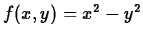$f(x,y) = x^2-y^2$ has a stationary point at the origin, but it is not a local extremum.

Finding and classifying the local extreme values of a function $f(x,y)$ requires several steps. First, the partial derivatives must be computed. Then the stationary points must be solved for, which is not always a simple task.

$$\frac{\partial f}{\partial x}=0=\frac{\partial f}{\partial y}$$

Next, one must check for the presence of singular points, which might also be local extreme values. Finally, each critical point must be classified as a local maximum, local minimum, or neither using the second-partials test

If $f_{xx}(a,b)f_{yy}(a,b)-[f_{xy}(a,b)]^2 >0$ and $f_{xx}(a,b) > 0$ then $f(a,b)$ is a local minimum.
If $f_{xx}(a,b)f_{yy}(a,b)-[f_{xy}(a,b)]^2 >0$ and $f_{xx}(a,b) < 0$ then $f(a,b)$ is a local maximum.
If $f_{xx}(a,b)f_{yy}(a,b)-[f_{xy}(a,b)]^2 <0$ then $f(a,b)$ is a saddle point.
If $f_{xx}(a,b)f_{yy}(a,b)-[f_{xy}(a,b)]^2 =0$ then no conclusion can be made.

Least Squares

The least-squares method is based on the line equation $y=mx+b$. Given data points, this method finds the line closest to all the data points. It does this by finding an m and b value such that the distance to the least-squares line is a minimum.

$$f(m,b)=d_{1}^2+d_{2}^2+...+d_{n}^2=\sum_{i=1}^n[y_{i}-(mx_{i}+b)]^2$$

Notice that the function to be minimized is a function of two variables and therefore the second-partials test will be used.

Exercises

Costs

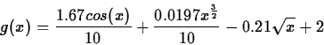
The costs that Shiela had in her ten years follows the following function:

$$g(x)=\frac{1.67cos(x)}{10}+\frac{0.0197x^{\frac{3}{2}}}{10}-0.21\sqrt{x}+2$$

A)

Enter the function.

B)

Plot the costs function over 120 months using the regular style=line. The income function fluxuates but follows an over-all linear path. This costs function fluxuates but does not follow an over-all linear path. Discuss a possible reason for this.

C)

To make a general comparison of normal buisness patterns at Shiela's station, what domain values would you include? Explain your reasoning. Then plot forty evenly-spaced data points in your domain.

D)

Enter the least-squares distance equation for the costs.

E)

Find a minimum point using all parts of the second-partials test to prove that the point is a minimum. Make sure to include plenty of text to keep your work clear.

F)

Using the minimum point that you found, write the line equation that will approximate the costs function.

G)

Graph data points of the original costs function along with the line equation that you just found over the full ten-year period. Make sure that your graph is clearly labeled.

Profits

For Shiela, to be a success, she not only wants her income to be larger than her costs but she also wants her profits to increase. Graph the difference between the income and the costs and explain whether Shiela is a success or not. Again, make sure your graph is clearly labeled.