


Next: About this document ...
Up: lab_template
Previous: lab_template
Subsections
To assist you, there is a worksheet associated with this lab that
contains examples. You can
copy that worksheet to your home directory with the following command,
which must be run in a terminal window, not in Maple.
cp /math/calclab/MA1024/Pardiff_grad_start.mws ~
For functions of two variables in Cartesian
coordinates, the graph is a set of points 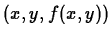 in
three-dimensional space. For this reason, visualizing
functions of two variables is usually more difficult.
The simplest way of describing a surface in Cartesian coordinates
is
as the graph of a function
in
three-dimensional space. For this reason, visualizing
functions of two variables is usually more difficult.
The simplest way of describing a surface in Cartesian coordinates
is
as the graph of a function  over a domain, e.g. a set
of
points in the
over a domain, e.g. a set
of
points in the  plane. The domain can have any shape, but a
rectangular one is the easiest to deal with.
Another way of representing a surface is through the use of level
curves. The idea is that a plane
plane. The domain can have any shape, but a
rectangular one is the easiest to deal with.
Another way of representing a surface is through the use of level
curves. The idea is that a plane  intersects the
surface in a curve. The projection of this curve on the plane
is
called a level curve. A collection of such curves for different values
of
intersects the
surface in a curve. The projection of this curve on the plane
is
called a level curve. A collection of such curves for different values
of  is a representation of the surface called a contour plot.
The partial derivatives
 and
and
 of
of  can be thought of as the rate of change of in
the direction parallel to the
can be thought of as the rate of change of in
the direction parallel to the  and
and  axes, respectively. The
directional derivative
axes, respectively. The
directional derivative
 , where
 is a unit vector, is the rate of change of in the
direction . There are several different ways that the
directional derivative can be computed. The method most often used
for hand calculation relies on the gradient, which will be described
below. It is also possible to simply use the definition
is a unit vector, is the rate of change of in the
direction . There are several different ways that the
directional derivative can be computed. The method most often used
for hand calculation relies on the gradient, which will be described
below. It is also possible to simply use the definition
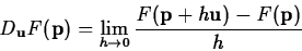
to compute the directional derivative. However, the following
computation, based on the definition, is often simpler to use.
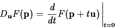
One way to think about this that can be helpful in understanding
directional derivatives is to realize that
 is
a straight line in the
is
a straight line in the  plane. The plane perpendicular to the
plane that contains this straight line intersects the surface
plane. The plane perpendicular to the
plane that contains this straight line intersects the surface  in a curve whose
  coordinate is
 . The derivative of
at
. The derivative of
at  is the rate of change of at
the point
is the rate of change of at
the point  moving in the direction .
The gradient of , written  , is most easily computed as
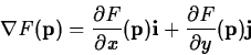
As described in the text, the gradient has several important
properties, including the following.
- Consider the following function.
- A)
- First, plot the graph of this function over the domain
 and
and
 using the plot3d
command. Then use the
contourplot command to generate a contour plot of
using the plot3d
command. Then use the
contourplot command to generate a contour plot of  over the same domain having 20 contour lines.
- B)
- What does the contour plot look like in the regions where the surface plot has a steep incline? What does it look like where the surface plot is almost flat?
- C)
- What can you say about the surface plot in a region whe
re the contour plot looks like a series of nested circles?
- Consider again the function from the first exercise. Using
either method from the Getting Started worksheet, compute the
directional derivative of at the point
 ,
,  in the
three directions below.
in the
three directions below.
- A)
-

- B)
-

- C)
-

- Using the method from the Getting Started worksheet,
plot the gradient field and the contours of on the same plot. Use
the domain of
 and
and
 . Use 20 contours and a 20 by 20 gradient field. Can you
use this plot to explain the values for the directional derivatives
you obtained in the previous exercises? By explaining the values, I
only mean can you explain what kind of surface it is and why the values were positive, negative, or zero in terms of the contours and the gradient field?
. Use 20 contours and a 20 by 20 gradient field. Can you
use this plot to explain the values for the directional derivatives
you obtained in the previous exercises? By explaining the values, I
only mean can you explain what kind of surface it is and why the values were positive, negative, or zero in terms of the contours and the gradient field?
Next: About this document ...
Up: lab_template
Previous: lab_template
Jane E Bouchard
2010-02-05