The first thing that you need to do is to open the DE toolbox.
> with(DEtools);

> eq:= diff(y(t),t) = sin(t)- 1/2*y(t);

> DEplot(eq,[t,y],t=0..12,{[0,0]},y=-3..3,title=`Figure0`);
The solution curve starts out at the point (0,0). Notice also that it is a little jagged. This can be smoothed out by forcing Maple to use more points in the solution (the default is 20). You can do this by specifying the stepsize:
> DEplot(eq,[t,y],t=0..12,{[0,0]},y=-3..3,stepsize=0.1,title=`Figure0: Smoother`);
You can put several solutions on the same graph by specifying several initial points.
> init:= seq([0,i],i=-3..3);

All of the solution curves, no matter what the initial position, seem to approach one single sine curve.
>DEplot(eq,[t,y],t=0..12,y=-3..3,arrows=THIN,title=`Figure2: A Direction Field`);
>DEplot(eq,[t,y],t=0..12,{[0,0]},stepsize=0.2,y=-3..3,arrows=THIN, title=`Figure 3`);
> dsolve(eq,y(t));

Warning: There are not many ODEs that have simple formulae for their solutions. This example was linear, so there is a nice solution formula. If you try to use dsolve on more complicated problems, especially noninear problems, Maple may give no answer, a really strange formula, or lock up your work station. (Remember the first rule of Maple: Save Early, Save Often!) Use dsolve with caution.
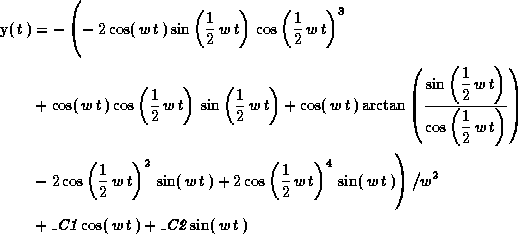
> eq2:= diff(y(t),t$2) + w^2*y(t) = sin(w*t);


© 1996 by Will Brother.
All rights Reserved. File last modified on October 1, 1996.