Overview. A graphical model is developed to reflect the structure of an ecosystem from a macroscopic viewpoint. It takes into account the manner in which energy/nutrients move through the food chain, dealing with the discrete relationships between members of the community as opposed to their dynamics. By utilizing the matrix associated with the graph, the overall structural nature of the ecosystem may be studied and the relative importance of each member of the community established. The graph is comparatively simple to set up and current software allows easy experimentation upon it.

Background Combinatoric Graphs (section 8.1 of Kolman or [10] ).

Introduction

The vast majority of quantitative models representing ecological systems are of a "local" nature, showing the dynamics of competing species, host-parasite, or some combination of the two. We say they are dynamic because they show how the population sizes change over time and whether the species under consideration persist in the long run. For the most  part, only a few species are modeled in part due the fact that data needed for parameters is difficult to obtain.

While work certainly has been done on the more overall, "global" nature of the ecosystem , e.g. [8] and [5], such work is infrequent as has not perhaps resulted in tools usable in the field by working biologists and ecologists due to the volume of data needed to make these models workable. In this material, an ecosystem is represented by a graph (in the mathematical sense of a collection of vertices and edges as opposed to a plot). This graph is straightforward to generate, easy to discuss as well as modify, and leads to valuable results concerning the relative importance of each specie in the community to the overall structural stability of the community.

A Graph of an Ecosystem

A directed graph representing the ecosystem under consideration is set up as follows:

   (1) for each species there is a node

   (2) there is a node for the environment itself

   (3) there is a directed line segment going from node i to node j

if the species associated with node j predates upon or  feeds off of the species of node i.

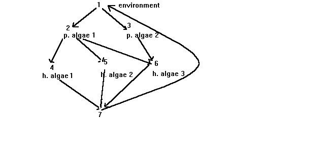
For example, suppose we have a pond with 2 species of photosynthetic algae, three species of herbaceous algae, and one bottom feeder. Then a graph consistent with above might look like:

where vertex 1 is for the environment; 2 and 3 for the photosynthetic algae etc. One may then view the arrows as showing how such resources as energy or particular nutrients flow through the ecosystem. The graph will probably change somewhat depending on what resource is being considered.

If, for example, the resource is energy, then at all levels, energy is being released back into the environment, so there would be additional arrows from each vertex back to vertex 1.

It is common to "label" graphs by associating something with each  arrow. In the context here, if a substance such as mercury were of interest,  a label might be established showing the relative concentration factor that occurs due to one specie feeding off of another. For example, if one type of fish fed off of another and a 5 fold increase in mercury resulted, then the arrow from the vertex of the prey to the predator could be labeled with a 5.

The graph described is then

        (1) straightforward to set up

        (2) provides macroscopic information about the structure of the ecosystem

        (3) can be a concise tool for communicating information about an ecosystem

        (4) does not require vast amounts of difficult to obtain data concerning individual species               population dynamics.

The graph could certainly be constructed by hand although in complex cases, one can envision applying the software power provided by a geographic information system (GIS) so that geographic relationships might also be incorporated.

It should be mentioned that graphs have been used before to represent relationships in ecosystems; an example is [10]. However in that paper, the graph was concerned with competition (an edge being constructed between two vertices if the two associated species competed with one another).

The Matrix of a Graph.

A great deal may be deduced about the structure of the ecosystem through its graph. However, the graph by itself has most of its value as a pictoral entity; analysis of it is often done with its associated "adjacency matrix" (if the graph has n vertices then its adjacency matrix, A, is nxn with entries defined as

          a_ij = 1 if an arrow goes from vertex j to i

                  0 otherwise

hence for the graph defined above, the adjacency matrix is

Three entities associated with the matrix of a graph are of potential value in the study of an ecosystem:

      * the dominant eigenvalue

      * an eigenvector of the dominant eigenvalue

      * powers of the matrix.

In this section we examine and justify each. As a starting point, we note that for such a graph and matrix,

       * the n row sums (sum of entries in each row) tell us many different species each specie has as           food sources

       * the n column sums tell us how many species each specie serves as possible food sources for.

We propose using the dominant eigenvalue of the adjacency matrix as a measure of the structural diversity of the ecosystem. (The dominant eigenvalue for such a nonegative matrix is the eigenvalue of largest absolute value. The Perron-Frobenius Theorem for nonegative matrices tells us that it is positive and has a positive associated eigenvector. Two results from linear algebra support such an interpretation:

     * the dominant eigenvalue lies in between the smallest and largest row sums or columns sums         (which ever bound is tighter)

    * if an entry in a nonegative matrix is increased then the dominant eigenvalue also increases.

The dominant eigenvalue is easy to compute and thus provides a concise measure of an important attribute of the ecosystem. In the above example,  the dominant eigenvalue is 1.748.

Next, by using standard graph theoretical notions (see [1], for example), one may examine powers of the matrix A with the information that

* the i,j th entry of A^k is the number of different paths from vertex i to vertex j of length k (by length of a path we mean the number of arrows in it).

This is useful information about the structure of the ecosystem. The more paths there are leading to a given specie, the less vulnerable that specie is to starvation due to the loss of a specie in the chain prior to it; it simply has alternative feeding opportunities. In particular, species with only a single path leading to them may be considered to be highly vulnerable. Similarly, a specie with only one path leading from it in the graph may be particularly valuable.

In the above example, one computes that A³ is

and thus, for example, that there are 4 different paths for food (or nutrients or energy, depending on what is under consideration) to go from the environment to species 7.

In general, suppose an ecosystem has r trophic levels and that the very last level has q different species in it. Then based upon the above discussion, if one looks at the first column of the matrix A^r, then the sum of the last q entries in that column should show how many different food chains there are through the entire ecosystem.

Associated with the positive, dominant eigenvalue of the adjacency matrix is a positive eigenvector (since a scalar multiple of an eigenvector is also an eigenvector, we are actually referring to any representative).  It is the purpose of this section to explore an interpretation of that vector in the context of an ecosystem.

The dominant eigenvector has n components; one for each species in the ecosystem as well as one for the environment. These components may have the interpretation of showing, for a given species relative to other species, how many food paths pass through it. We establish this mathematically as follows.

If u denotes an n dimensional column vector with one for all entries, so that u = (1, 1, 1, . . . 1)^t

then the column Au has the row sums of A as entries, and similarly, A^k u has the rows sums of the kth power of A as entries. Taking the previous discussion into account, A^k u has as its ith entry the number of food paths to specie i of length k or less. If we examine the components of the vector

               lim A^k u

                 k->oo

it shows the number of paths going to each specie of any length. While the actual components of this vector have no meaning, the values relative to one another do, showing the flow to each member of the community.

Now mathematically it may be shown (see project 5 )that the vector A^k u becomes the dominant eigenvector of A as k becomes large. In the simple ecosystem above, this vector (or any scalar multiple of it) is

    (.592 , .338,.338,.194,.194,.387,.443)^t

The 4th, 5th and 6th components show for the corresponding species that species 6 has twice the feeding opportunities that species 4 and 5 do.

Conclusion

A graph may be easily set up to visually show nutrient flow between the species comprising a community. Additionally, by examining the associated matrix of this graph, an overall measure of diversity of flows throughout the ecosystem may be obtained (the dominant eigenvalue), the number of paths from one specie to another may be calculated by powers of the matrix, and the relative flow to any specie may be obtained by comparing components of the dominant eigenvector. These results then provide a quantitative measure for describing the macroscopic structure of an ecosystem.

Problems

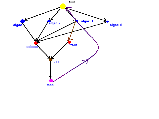
Suppose an ecosystem is represented graphically as:

Using linear algebraic techniques, decide which species in the ecosystem are critical to the stability of the system, and which are not.

Suppose that the salmon are economically important to the area that it resides in (true in the Pacific Northwest, for example). If there are pollutants entering the waters which threaten some of the algae, which ones are most critical to the welfare of the salmon? Can you demonstrate this mathematically? What are the dominant eigenvalue and eigenvector of this ecosystem? How would you interpret them? If the salmon can no longer consume algae 3 and 4, how do your computations change? Are the new numbers reflective of the changes made in the ecosystem?

In general, how would you interpret the dominant eigenvalue of the ecosystem? Suppose, for sake of discussion that we have two different ecosystems with the same number of species. The first one has a dominant eigenvalue of 2.8 while the second one has a dominant eigenvalue of 1.4. How would you compare them?

References

1. Chartrand, G.,1977 Graphs as Mathematical Models, Prindle,Weber & Schmidt, Boston,     Massachusetts,7.

2. Gould, Peter. 1967. The Geographic Interpretation of Eigenvalues.Transactions of the Institute     of British Geographers 42: 53-85.

3. Hutchinson, G. Evelyn 1978. An Introduction to Population Ecology. . New Haven: Yale     University Press.

4. Kormondy, E.J.,1969 Concepts of Ecology, Prentice-Hall, Englewood Cliffs, New Jersey,

5. May, R.M., 1973 Stability and Complexity in Model Ecosystems, Princeton University Press,     Princeton, New Jersey.

6. Minc, H.,1988 Nonegative Matrices, John Wiley & Sons, New York, New York .

7. Paine, R.T., Food Web Complexity and Species Diversity, American Naturalist, 100:65-75     (1966).

8. Pielou, E.C.,1975 Ecological Diversity, John Wiley & Sons, New York, New York .

9. Pielou, E.C.,1969 An Introduction to Mathematical Ecology, John Wiley & Sons, New York,     New York.

10. Roberts, F.S., Graph Theory and Its Application to Problems of Society, NFS-CBMS      Monograph No. 29, SIAM, Philadelphia, PA, 1978

11.Straffin, Philip D. 1980. Linear Algebra in Geography: Eigenvectors of Networks. Mathematics      Magazine 53(5): 269-276.

12. Varga, R.S.,1962 Matrix Iterative Analysis, Prentice-Hall, Englewood Cliffs, New Jersey.