I. Introduction

The purpose of this project is to gain understanding and experience with the notion of expanding a function as a Fourier Series. This powerful method is at the heart of applications in mechanics, sound, signal processing, image processing, and many other areas of modern science and engineering. It goes hand in hand with the Fourier Transform, whose roots lie in optics.

II. Background

 Review class notes on orthogonal basis or the textbook for MA 2051, Differential Equations by Professor Davis, specifically section 9.4

Recall from earlier in the course our discussions on changes of coordinate systems. In general, finding the coordinates of a vector in a new coordinate system amounted to straightforward solution of a linear system. We also showed if the new coordinate system was orthogonal, then solving for the new coordinates of a given vector was far easier; one could isolate each coefficient via dot products instead of solving a system of equations. That concept lies at the heart of Fourier Series.

Our problem here is to take an arbitrary function f(x) defined and finite on the for x between -1 and +1 and to expand it in terms of the orthogonal basis

                         { 1, cos(px), cos(2px), cos(3px),. . . , sin( px), sin(2px),sin(3px). . . }

such an expansion is called a Fourier Series of the function f. The coefficients, rather than being called coordinates, are called Fourier coefficients, but the concept is identical.

Maple Review

In order to do this work, the reader will need to be able to use software to

1. Define a function

2. Do a definite integral

3. Plot a function or functions

Three brief examples should suffice for those using Maple:

> f:= x-> x^2 + cos(2*x) +2*Pi;                 defines a function f(x)=x² + cos(2x) +2p

and

> a:= int(f(x),x=-2..2);                                performs the definite integral of f and assigns it to a

while

> plot({f(x),g(x)},  x=0..5};                            plots f(x) and g(x) on the same graph, for 0<x<5

Part One Establishing the Orthogonality of the Basis

{ 1, cos(px), cos(2px), cos(3px),. . . , sin( px), sin(2px),sin(3px). . . }

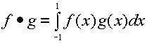
First we must define a "dot product" of two functions. We define it as:

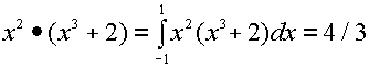
so, for example,

(In most material on Fourier Series, this is called an inner product instead of dot product).

Having done this, we may work on the problem at hand, pointing out that there are really five dot products which must be shown to be 0 so that all possibilities are covered. For example, we must show

as well as three others (what are they?). Use Maple to establish all 5 results.

Part Two Expanding a function in a Fourier Series

if f(x) = a₀ + a₁ cos(px) + a₂ cos(2px) + . . . + b₁sin(px) + b₂ sin(2px) + b₃ sin(3px). .

our problem is to find the coefficients a₀, a₁,a₂. . . b₁, b₂,. . . This is greater aided by the orthogonality you established in Part One. Just as in the case of geometric vectors, we may take the dot product first of both sides with 1:

f(x) · 1 = 1 · (a₀ + a₁ cos(px) + a₂ cos(2px) + . . . + b₁sin(px) + b₂ sin(2px) + . .)

            = 1· a₀ by the orthogonality!

            = 2 a₀  ,           so we can solve for a₀

similarly, taking the dot product of both sides with cos(npx) gives

f(x) · cos(npx) = cos(npx) · (a₀ + a₁ cos(px) + a₂ cos(2px) + . . . + b₁sin(px) + b₂ sin(2px) + . . .)

                           = cos(npx) · a_n cos(npx) by the orthogonality!

                           = a_n by direct integration

so a_n is easily solved for.

Finally, one may take the dot product of both sides with sin(npx) and isolate b_n in a like manner. Since we have treated n as a parameter, rather than a specific value, we have covered all cases and have the Fourier Series of f(x)

For example, we find the Fourier Series of the function f(x) = x² -3x + 1. By direct integration, we find that

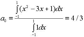
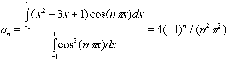
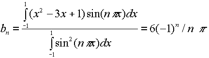
so

x² -3x + 1 = 2/3 -(4/ p²)cos(px)+(4/4 p²)cos(2px)- (4/9 p²)cos(3px)...-6/psin((px)+ (6/2 p) sin(2px)-

(6/3 p) sin(3px) . . .

Exercises: 

1. Find the Fourier Series for each function below, whose definition for -1 < x < +1 is:

a. f(x) = 2x+1                   b. f(x) = 7cos(2px)                          c. f(x) = x³ + x²+ 1

( you should have a formula for a_n and b_n in each case and also write out the first 4 nonzero terms if possible)

2. For the function in 1a above, on the same graph, plot it as well as

a. the first two nonzero terms of the Fourier Series for it

b. the first three nonzero terms of the Fourier Series for it

c. the first four nonzero terms of the Fourier Series for it

(so you should hand in 3 graphs altogether)

3. Prove (on paper, not Maple) that if f(x) is an even function (symmetric about the y axis; f(-x) = f(x) ) then b_n = 0 for all n

    Include 3 examples of even functions.

4. Prove that if f(x) is an odd function (antisymmetric about the y axis; f(-x) = -f(x) ) then a_n = 0 for all n

    Include 3 examples of odd functions.

5. Compare Fourier Series and Taylor Series (MA1023). When can each be used? What sorts of functions can be expanded in a Fourier Series? In a Taylor Series? Consider as a point of discussion the function f(x) defined on -1< x < +1 by f(x) = 0 if x < 0 and f(x) = 1 if x > 0 (a "step function"). Can a Taylor Series be found for it? a Fourier Series? You may want to use an outside reference book to look up conditions for each kind of series being applied.

6. Each person in your team should speak with a faculty member in the department of your major and learn about one application of Fourier Series. Include this information in your document to be turned in.