Introduction The purpose of this project is to gain an introduction into regression analysis and how linear algebra relates to it. Regression analysis is concerned with taking data points and fitting the best possible curve one can to them. In this lab, we will look at the mathematics behind this as well as how Maple may be used to provide graphical as well as computational assistance. We will study both linear regression analysis (fitting straight lines to data) as well as some non linear regression analysis

Real life situations rarely have perfect equations describing them, nor well known constants associated with them. One often has to gather data and make estimates. Regression analysis is a time tested and powerful tool in this context, for people in all fields: science, engineering, management and social science.

For practical applications, one usually uses a statistical package such as SPSS to perform the calculations. Here we are trying to see the mathematics behind the computations, in particular how it uses calculus and linear algebra to determine best fits. Using SPSS is much quicker but shows none of the mathematics associated with the calculations.

Background: Using Maple to Plot Data Points and Curves

(If your team has chosen another package instead of Maple, disregard all Maple commands in what follows).

In this section, the goal is to try out Maple commands to plot data points and curves on the same plot graph. Many of you have probably plotted curves and surfaces in other courses. Adding data points to this takes a few more commands.

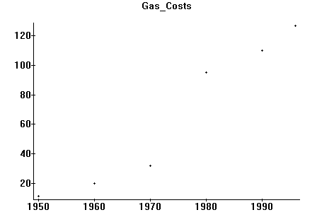
Suppose we are looking at the cost of a gallon of gasoline over the last half century. We obtain data:

1950 :11cents   1960: 20    1970: 32    1980: 90    1990: 110    1996:127

which we wish to plot on a 2 dimensional graph. The steps in Maple would be as follows:

  >with(plots); invoke "plots" library

  >datalist:= [[1950,11] , [1960,20], [1970,33], [ 1980,90],[1990,110],[1996,127]];

  >pointplot:=plot(datalist,style=POINT,title=‘Gas_Prices’): (note the colon!)

  >display(pointplot); (should plot them in a window)

Remarks: the names "datalist" and "pointplot" are entirely up to the user! Also the title of the graph, "Gas_Prices" cannot have any spaces in it (hence I used an underscore). 

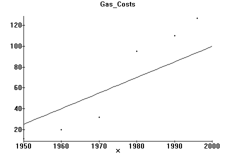
Next, lets assume we wanted to also plot a straight line on top of this. For sake of discussion, let’s say we wanted to plot the straight line

                                y = 1.5 x - 2900 (x in units of years, y in cents)

on the same graph as above. To do this requires 2 steps, first storing the plot in a data structure I’ll call "curveplot" and then graphing it along with the data from above on a graph. The Maple commands to do this might appear as:

  > curveplot:=plot(1.5*x - 2900,x=1950..2000): (note the colon again)

  >display([pointplot,curveplot]); (show both!)

 resulting in:

PART ONE: Linear Regression Analysis 

This means finding the straight line which best fits the data. Now clearly no straight line can go exactly thru all 5 points unless they were collinear, which they aren’t. Thus every straight line will have an error associated with it. We will seek to minimize that error (which we have yet to define!). 

Before that, however, by trial and error, find the straight line which you feel best fits the above data from a visual perspective (i.e. the plot of both). Do this by plotting both the data and straight line, as above, and then experimenting with both the slope and intercept of the line until you feel it looks the best. Record this equation and include it in the write up of this project.

Next calculate the error associated with your straight line according to the following formula:

where the sum is over all 5 data points. Here a is your slope, b your y intercept, and (x_i,y_i) is the coordinate of the ith data point (so (x₁,y₁) = (1950,11) etc). Record this calculation for your write up.

The error expression, E, above, will be used in all parts of this project. Only the function, in this case ax_i + b, will change.

What does E mean or tell us? You are taking the difference of the y value of the data point and the y value of the straight line (so the vertical difference, or error), squaring it and adding them all up. The square is so errors don’t cancel each other out due to sign differences. Thus E can be interpreted as the total error of the straight-line (there are other possible definitions).

What does your straight-line predict for the year 1995? 2000? (this is called extrapolation).

The "best" straight line

Finding a good straight line fit, as you have done by trial and error is ok for a few data points but impractical for large numbers. Here we use calculus to develop a more general method. Note the total error, E, as defined above, has two variables to determine it, the slope a and the intercept b (the x_i and y_i are constants). Thus we seek to find values for a and b that minimize E. This should sound familiar from calculus!

We do this by taking the derivatives of E with respect to both a and b, and setting them equal to 0.

(Here, we have used the power rule and the fact that the derivative of a sum is the sum of the derivatives). Please take time to check why the above derivatives come out as they do as you will need it for a later portion of the project.

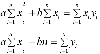
Next, show algebraically that the above two equations are equivalent to the system of 2 equations and two unknowns (a,b):

Note n is the number of data points, 5 in the example earlier.

The situation is now that we have two linear equations and two unknowns (a and b). Please set up the two equations as they should be for the data above, solve the system, and write down the straight line equation you get. Also plot it on the same graph as the data and your best "guess" straight line. Finally, compute the total error associated with the optimal straight line you just finished finding. How does it compare with the total error you have already calculated for your best "guess" straight line? Include all of this in the write up of the project.

The straight line generated by the above process is called the "least squares linear fit". The "least squares" refers to picking it so the error is minimized, where the error was the sum of the squares of the pointwise errors.

PART TWO: Nonlinear Regression Analysis - quadratic and cubic fits

The above generation of a straight line is useful but only if the data that one has seems to follow a linear pattern. Also, one need not invoke Maple to perform it; many calculators have all the software built in to generate a and b if the data points are entered. 

Sometimes data is clearly nonlinear, the simplest example being parabolic or quadratic in appearance. Consider the rising cost of health care. The following data is per capita spending in the U.S.,1960-1995:

1960 $143   1965 $204   1970 $346   1975 $600   1980 $1059  1985 $1700   1990 $2550   1995 $3225

Please include the following in your writeup:

      a. a plot of the data

      b. pick a parabola you feel best fits it from a graphical view (trial and error, as above)

                                      form: y = ax² + bx + c

      c.set up the total error function for a parabola. Find the system of 3 equations which result from setting 3 partial       derivatives equal to zero. The parabola which results is called the "least squares quadratic fit"

     d. Solve the system of 3 equations &unknowns for the data just presented. How does your "best fit" parabola compare to      your own? How do the total errors compare? Include this in your report.

     e. What does your work predict for the per capita cost in 1997? 1998? 2000?

Cubic Fits: Suppose your data appeared to be cubic, or you knew in advance that it was. For example, if one gathered data from a wind tunnel test of a car on the horsepower needed to go a given velocity, the relationship is known to be cubic (the horsepower needed going up with the cube of the velocity).

A general cubic function is given by

                               y = a x³ + b x² + cx + d

in this section ,please

     a. set up the total error function for the above cubic

     b. take the partial derivatives wrt to all 4 parameters

     c. show what the system of equations is that will result in solutions for the 4 parameters for the "least squares cubic fit "

     d. Suppose from wind tunnel tests a car requires the following amounts of horsepower to go the stated speeds: 9 hp for 45 mph, 12 hp for 55 mph, and 17 hp for 65 mph. Fit a cubic to this data

     e. According to your curve, how much horsepower will be needed to go 75 mph?

If gas mileage is inversely proportional to horsepower used, how much of a decrease will result in gas mileage at 75 mph vs 65?

PART FOUR Calculators.

Most calculators will perform at least linear regression analysis. Find your manual for your calculator and review both its capabilities and how to actually use it. Which of the problems above could be done with your calculator? Pick one and do it.

Include in your report what calculator each person in the team has and what it has for regression analysis capabilities.

Additionally, is your calculator capable of generating a "correlation coefficient", perhaps called "r" in the display on the calculator? If so, do you have any sense of what this is for?