The linalg package in Maple contains four commands that may be useful. Assume A is n by n matrix.
> eigenvals(A);
- - this gives the eigenvalues of A.
> eigenvects(A);
- - for each eigenvalue, this command returns the eigenvalue, its algebraic multiplicity, and a basis for its eigenspace.
> charmat(A,lamda);
- - this yields the matrix ![]() .
.
> charpoly(A,lamda);
- - this produces the characteristic polynomial.
Maple's online help contains more information about these commands.
Consider an example of an animal population whose size is determined by characteristics of the female. (The assumption is that there will always be enough males to propogate the species.) Suppose the maximal lifespan of the females is three years. On the average, 37% of the newborns live to be one year old and 30% of the one-year olds live to be two years old. Further, on the average, each one-year old produces 3 female offspring and each two-year old produces 1 female offspring. Let ![]() be the column 3-vector that gives the number of females in the three age groups in year k. Then
be the column 3-vector that gives the number of females in the three age groups in year k. Then ![]() where
where 
Such a population model is called a Leslie model and A is a Leslie Matrix. In general,

where ![]() is the number of offspring per individual in group i and
is the number of offspring per individual in group i and ![]() is the probability that an individual in group i survives one period to become a member of group i + 1.
is the probability that an individual in group i survives one period to become a member of group i + 1.
A
It can be shown that a Leslie matrix has a unique positive eigenvalue, say ![]() , that is simple (not repeated) and dominant, i.e,
, that is simple (not repeated) and dominant, i.e, ![]() for j > 1. Further, under mild conditions on the matrix,
for j > 1. Further, under mild conditions on the matrix, ![]() is strictly dominant, i.e.,
is strictly dominant, i.e., ![]() for j > 1. In this case,
for j > 1. In this case, ![]() and
and ![]() for large k, where
for large k, where ![]() is an eigenvector corresponding to
is an eigenvector corresponding to ![]() . (To see the first assertion, divide both sides of the equation
. (To see the first assertion, divide both sides of the equation ![]() by
by ![]() and let k get large; the second assertion follows from the first.) Thus
and let k get large; the second assertion follows from the first.) Thus ![]() gives the long-term growth rate per time period, and from
gives the long-term growth rate per time period, and from ![]() we get the long-term proportions of the population in the different age groups.
we get the long-term proportions of the population in the different age groups.
Section 11.18 of the text contains a more extensive discussion of this topic.
Suppose A is a stochastic (or Markov or probability) matrix, i.e., each entry of A is nonnegative and the sum of the entries in any column of A is 1. A process described by such an A is a Markov process or Markov chain and A is a transition matrix.
It can be shown that 1 is a dominant eigenvalue of A, i.e., ![]() for all j. Further, it often happens that one eigenvalue, say
for all j. Further, it often happens that one eigenvalue, say ![]() , is 1 and all other eigenvalues
, is 1 and all other eigenvalues ![]() satisfy
satisfy ![]() . Then 1 is a strictly dominant eigenvalue of A, and it follows that
. Then 1 is a strictly dominant eigenvalue of A, and it follows that ![]() as
as ![]() (because
(because ![]() for j > 1).
for j > 1).
If the sum of the coordinates of each ![]() is 1, then
is 1, then ![]() approaches that eigenvector corresponding to eigenvalue 1 whose coordinates sum to 1; this limit is the steady state of the Markov process. Thus, rather than finding
approaches that eigenvector corresponding to eigenvalue 1 whose coordinates sum to 1; this limit is the steady state of the Markov process. Thus, rather than finding ![]() , we can simply scale
, we can simply scale ![]() and the result will be the limit of
and the result will be the limit of ![]() .
.
Some discussion of Markov chains is given in Section 11.6 of the text. Take special note of Theorem 11.6.4.
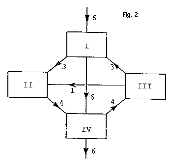
Systems of linear differential equations arise in a variety of ways. The study of spring-mass systems or investigations in control theory can lead to such systems. Exercise 3 below is a mixing problem. This same technique might be used to study the flow of a substance through the body. Section 9.1 of the text deals with solutions of systems of linear differential equations. Note well the role of initial conditions in such solutions.
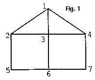
Let ![]() be the column 7-vector of probabilities that the guard is at intersections
be the column 7-vector of probabilities that the guard is at intersections ![]() after k 15-minute time periods.
after k 15-minute time periods.

