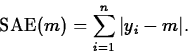
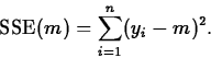
The validity of inference is related to the way the data are obtained, and to the stationarity of the process producing the data.
For valid inference the data must be obtained using a probability sample. The simplest probability sample is a simple random sample (SRS).
![]()
Recall the example from Chapter 4:
One stage of a manufacturing process involves a manually-controlled
grinding operation. Management suspects that the grinding machine
operators tend to grind parts slightly larger rather than
slightly smaller than the target diameter, 0.75 inches while still
staying within specification limits, which are 0.75 ![]() 0.01 inches.
To verify their suspicions, they sample 150 within-spec parts. Summary
measures and graphs are displayed on the following output.
0.01 inches.
To verify their suspicions, they sample 150 within-spec parts. Summary
measures and graphs are displayed on the following output.
We will assume these data were generated by the C+E model:
![]()
The distribution model of an estimator is called its sampling
distribution. For example, in the C+E model, the least squares
estimator ![]() , has a
, has a ![]() distribution (its
sampling distribution):
distribution (its
sampling distribution):
A level L confidence interval for a
parameter ![]() is an interval
is an interval ![]() , where
, where ![]() and
and ![]() are
estimators having the property that
are
estimators having the property that
![]()
Confidence Interval for ![]() : Known Variance
: Known Variance
Suppose we know ![]() . Then if
. Then if ![]() can be assumed to
have a
can be assumed to
have a ![]() sampling distribution, we know that
sampling distribution, we know that
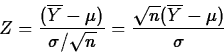
Noting that
![]()
Denoting the standard error of ![]() ,
, ![]() , by
, by
![]() , we have the formula
, we have the formula
![]()
The confidence level, L, of a level L confidence interval for a
parameter ![]() is interpreted as follows: Consider all possible
samples that can be taken from the population described by
is interpreted as follows: Consider all possible
samples that can be taken from the population described by ![]() and for each sample imagine constructing a level L confidence
interval for
and for each sample imagine constructing a level L confidence
interval for ![]() . Then a proportion L of all the constructed
intervals will really contain
. Then a proportion L of all the constructed
intervals will really contain ![]() .
.
Recall again the example from Chapter 4:
One stage of a manufacturing process involves a manually-controlled
grinding operation. Management suspects that the grinding machine
operators tend to grind parts slightly larger rather than
slightly smaller than the target diameter, 0.75 inches while still
staying within specification limits, which are 0.75 ![]() 0.01 inches.
To verify their suspicions, they sample 150 within-spec parts. Summary
measures and graphs are displayed on the following output.
0.01 inches.
To verify their suspicions, they sample 150 within-spec parts. Summary
measures and graphs are displayed on the following output.
We will assume these data were generated by the C+E model:
![]()
![]()
![]()
=(0.7518-(0.0004)(1.96),0.7518+(0.0004)(1.96))
=(0.7510,0.7526).
Based on these data, we estimate that ![]() lies in the interval
(0.7510,0.7526). As all values in this interval exceed 0.75, we
conclude that the true
mean diameter,
lies in the interval
(0.7510,0.7526). As all values in this interval exceed 0.75, we
conclude that the true
mean diameter, ![]() , is greater than 0.75. We are 95% confident in
our conclusion, meaning that in repeated sampling, 95% of all
intervals computed in this way will contain the true value of
, is greater than 0.75. We are 95% confident in
our conclusion, meaning that in repeated sampling, 95% of all
intervals computed in this way will contain the true value of ![]() .
.
Classical Confidence Interval for
![]() : Unkown Variance
If
: Unkown Variance
If ![]() is unknown, estimate it using the sample standard
deviation, S. This means that instead of computing the exact
standard error of
is unknown, estimate it using the sample standard
deviation, S. This means that instead of computing the exact
standard error of ![]() , we use the estimated standard error,
, we use the estimated standard error,
![]()
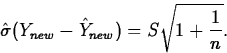
However, the resulting standardized estimator,

![]()
Recall the example from Chapter 4:
For these data, n=150 and s=0.0048, which means that
![]() .In addition,
.In addition, ![]() ,so a level 0.95 confidence interval for
,so a level 0.95 confidence interval for ![]() is
is
(0.7518-(0.0004)(1.976),0.7518+(0.0004)(1.976))
=(0.7510,0.7526).
This interval is identical (to four decimal places) with the interval computed assuming
The problem is to predict a new (i.e. not yet available) observation
from the C+E model using presently available data. To see what is
involved, suppose we know ![]() . Then it can be shown that we should
predict the new observation to be
. Then it can be shown that we should
predict the new observation to be ![]() . However, even using this
knowledge, we will still have prediction error:
. However, even using this
knowledge, we will still have prediction error:
![]()
We won't know ![]() , however, so we estimate it from the present data
by computing
, however, so we estimate it from the present data
by computing ![]() , and use this as the predictor
of the new observation. When
, and use this as the predictor
of the new observation. When ![]() is used for prediction
instead of estimation, we call it
is used for prediction
instead of estimation, we call it ![]() . When using
. When using
![]() to predict a new observation, the prediction error is
to predict a new observation, the prediction error is
![]()
![]() is the error due to using
is the error due to using ![]() to estimate
to estimate
![]() . Its variance, as we have already seen, is
. Its variance, as we have already seen, is ![]() .
.![]() is the random error inherent in Ynew. Its
variance is
is the random error inherent in Ynew. Its
variance is ![]() . Since these terms are independent, the
variance of their sum is the sum of their variances.
. Since these terms are independent, the
variance of their sum is the sum of their variances.
In most applications ![]() will not be known, so we estimate it
with the sample standard deviation S, giving the estimated standard
error of prediction
will not be known, so we estimate it
with the sample standard deviation S, giving the estimated standard
error of prediction
A classical level L prediction interval for a new observation is then
![]()
We return to the grinding example from Chapter 4.
Recall that for these data, ![]() , so that the
predicted value is
, so that the
predicted value is ![]() . Also,
n=150 and s=0.0048, which means that
. Also,
n=150 and s=0.0048, which means that
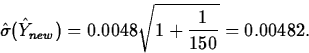
(0.7518-(0.00482)(1.976),0.7518+(0.00482)(1.976))
=(0.7422,0.7614).
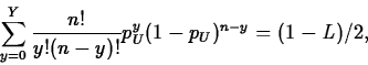
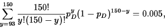
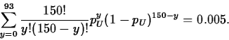
Exact Confidence Interval for p
Suppose we observe Y successes in the n trials. Then a level L confidence interval for p is (pD,pU), where
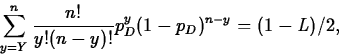
and
Classical Estimation for Large Samples
Suppose ![]() , where n is large (rule of thumb: Y
and n-Y exceed 10). Let
, where n is large (rule of thumb: Y
and n-Y exceed 10). Let ![]() be the sample proportion of
successes, and let
be the sample proportion of
successes, and let ![]() be its estimated standard error. Then by the CLT,
be its estimated standard error. Then by the CLT,
![]()
![]()
(0.62-(0.0396)(2.5758),0.62+(0.0396)(2.5758))
=(0.52,0.72).
As can be seen, in this case both intervals agree closely. In particular, as each interval contains only values exceeding 0.5, we can conclude with 99% confidence that more than half the population diameters exceed spec.
One consideration in designing an experiment or sampling study is the precision desired in estimators or predictors. Precision of an estimator is a measure of how variable that estimator is. Another equivalent way of expressing precision is the width of a level L confidence interval. For a given population, precision is a function of the size of the sample: the larger the sample, the greater the precision.
Suppose it is desired to estimate a population proportion p to within d units with confidence level at least L. If we assume a large enough sample size (so the normal approximation can be used in computing the confidence interval), the requirement is that one half the length of the confidence interval equal d, or
![]()
![]()
There is an analogous formula when a simple random sample will be used
and it is desired to estimate a population mean ![]() to within d
units with confidence level at least L. If we assume a large enough
sample size (so the normal approximation can be used in computing the
confidence interval), the required sample size is
to within d
units with confidence level at least L. If we assume a large enough
sample size (so the normal approximation can be used in computing the
confidence interval), the required sample size is
![]()
We assume that there are n1 measurements from population 1 generated by the C+E model
![]()
![]()
We want to compare ![]() and
and ![]() .
.
Sometimes each observation from population 1 is paired with another
observation from population 2. For example, each student may take a pre-
and post-test. In this case n1=n2 and by looking at the pairwise
differences, Di=Y1,i-Y2,i, we transform the two population
problem to a one population problem for C+E model
![]() , where
, where ![]() and
and
![]() . Therefore, a confidence interval
for
. Therefore, a confidence interval
for ![]() is obtained by constructing a one sample confidence
interval for
is obtained by constructing a one sample confidence
interval for ![]() .
.
The manufacturer of a new warmup bat wants to test its efficacy. To do
so, it selects a random sample of 12 baseball players from among a
larger number who volunteer to try the bat. For each player, company
researchers
compute D, the difference between the player's test year average
and his pervious year's average. Assuming that these differences
follow a C+E model, they construct a level 0.95
confidence interval for the difference in mean batting average,
![]() .The data (found in SASDATA.BATTING) are:
.The data (found in SASDATA.BATTING) are:
| PLAYER | BEFORE | AFTER | DIFF |
| 1 | 0.254 | 0.262 | 0.008 |
| 2 | 0.274 | 0.290 | 0.016 |
| 3 | 0.300 | 0.304 | 0.004 |
| 4 | 0.246 | 0.267 | 0.021 |
| 5 | 0.278 | 0.291 | 0.013 |
| 6 | 0.252 | 0.257 | 0.005 |
| 7 | 0.235 | 0.248 | 0.013 |
| 8 | 0.313 | 0.324 | 0.021 |
| 9 | 0.305 | 0.317 | 0.012 |
| 10 | 0.255 | 0.252 | -0.003 |
| 11 | 0.244 | 0.276 | 0.032 |
| 12 | 0.322 | 0.332 | 0.010 |
An inspection of the differences shows no evidence of nonnormality or
outliers. For these data,
![]() , sd=0.0092 and t11,0.975=2.201.
Then
, sd=0.0092 and t11,0.975=2.201.
Then ![]() , so the
desired interval is
, so the
desired interval is
![]()
Let ![]() and
and ![]() denote the sample
means from populations 1 and 2,
S12 and S22 the
sample variances.
The point estimator of
denote the sample
means from populations 1 and 2,
S12 and S22 the
sample variances.
The point estimator of ![]() , is
, is
![]() .
.
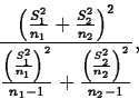
If the population variances are equal
(![]() ), then
we estimate
), then
we estimate ![]() by the pooled variance estimator
by the pooled variance estimator
![]()
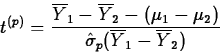
![]()
If ![]() , an approximate level L confidence
interval for
, an approximate level L confidence
interval for ![]() is
is
![]()
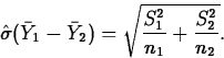
A company buys cutting blades used in its manufacturing process from two suppliers. In order to decide if there is a difference in blade life, the lifetimes of 10 blades from manufacturer 1 and 13 blades from manufacturer 2 used in the same application are compared. A summary of the data shows the following (units are hours):
| Manufacturer | n | s | |
| 1 | 10 | 118.4 | 26.9 |
| 2 | 13 | 134.9 | 18.4 |
The experimenters generated histograms and normal quantile plots of
the two data sets and found no evidence of nonnormality or outliers.
The estimate of ![]() is
is ![]() .
.
![]()
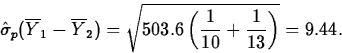
![]()
=(-32.7,-0.3).
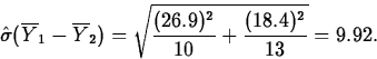
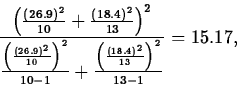
![]()
=(-33.9,0.89).
![]() and
and ![]() are observations from
two independent populations. Estimator of p1-p2 is
are observations from
two independent populations. Estimator of p1-p2 is
![]()
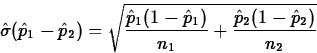
![]()
In a recent survey on academic dishonesty 26 of the 200 female college students surveyed and 26 of the 100 male college students surveyed agreed or strongly agreed with the statement ``Under some circumstances academic dishonesty is justified.'' With 95% confidence estimate the difference in the proportions pf of all female and pm of all male college students who agree or strongly agree with this statement.
The point estimate of pf-pm is
![]()
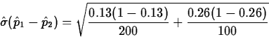
=0.05.
Since Yf=26, 200-Yf=174, Ym=26, and 100-Ym=74 all exceed 10, we may use the normal approximation, which gives the interval(-0.13-(0.05)(1.96),-0.13+(0.05)(1.96))
=(-0.228,-0.032).
Tolerance intervals are used to give a range of values which, with a
pre-specified confidence, will contain at least a pre-specified
proportion of the measurements in the population. Suppose T1 and
T2 are estimators with ![]() , and that
, and that ![]() is a real
number between 0 and 1. Let
is a real
number between 0 and 1. Let ![]() denote the event
denote the event
{The proportion of measurements in the population between T1
and T2 is at least ![]() }.
}.
Then a level L tolerance interval for a
proportion ![]() of a population is an interval
of a population is an interval ![]() , where T1 and T2 are estimators, having the property that
, where T1 and T2 are estimators, having the property that
![]()
If we can assume the data are from a normal population, a level L
tolerance interval for a proportion ![]() of the population is given by
of the population is given by
![]()
Refer again to the grinding data. The mean diameter of the n=150 parts is 0.7518 and the standard deviation is 0.0048. For level 0.90 normal theory tolerance interval for a proportion 0.95 of the data, the constant K is obtained by simple interpolation to be 2.137. The interval is then
![]()
![]()