$next$ $up$ $previous$

CHAPTER 7

THE RELATIONSHIP BETWEEN TWO VARIABLES

7.18.

Not necessarily. Blood pressure and income both tend to increase with age. (10 points)

7.22.

We have

$\begin{displaymath} \hat{\beta}_1 & = & r\frac{s_Y}{s_X}=r=0.90 {\bf (5 points)}\end{displaymath}$

$\begin{displaymath} \hat{\beta}_0 & = & \overline{y}-\hat{\beta}_1 \overline{x}= 13.07-(0.90)(12.82)=1.532 {\bf (5 points)}\end{displaymath}$

$\begin{displaymath} \hat{Y} & = & 1.532+0.90 X\end{displaymath}$

7.28.

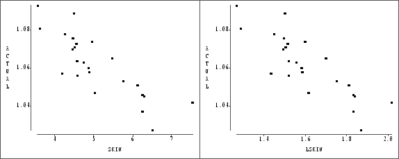
(a)

Shown are the graphs of ACTUAL versus SKIN and LSKIN. (10 points): 5 for each graph

$\psfig {file=exsol7_4.eps,height=2in,width=5in}$

Both plots show a decreasing linear relation. (5 points) There does not seem to be a reason to prefer one over the other. (5 points)

(b)

Both fits appear adequate with the regression of ACTUAL on LSKIN being preferred because of a slightly larger r² (0.6930 versus 0.6736) and slightly lower MSE (0.0093 versus 0.0096). There is little to choose from in graphs of the fits or in the residual plots. (10 points)

(c)

The fitted slope of the regression of ACTUAL on LSKIN is -0.0725. This means that for each unit increase in LSKIN, we lower our prediction of ACTUAL by 0.0725 units. (10 points)

(d)

Possibly. An LSKIN value of 0 corresponds to a SKIN value of 1, so if it is possible to have a skinfold measurement of 1, then the intercept, $\hat{\beta}_0=1.1781$ , is the prediction of body density at that skinfold value. Caution must be taken, however, in extrapolating beyond the range of the data. (5 points)

For the regression of ACTUAL on SKIN, not only is a skinfold value of 0 not in the data set, but, in fact, makes no sense. So the intercept has no interpretation in this case. (5 points)

7.38.

(a): $\widehat{VOLUME}=-36.9435+5.0659\cdot DIAM$ . The intercept has no physical meaning (what is a negative volume?). The slope of 5.0659 means that the model predicts that a tree with 1 inch greater diameter will have 5.0659 ft³ more volume.
(b): The model under-predicts volume for large and small diameters and over-predicts for intermediate diameters. A transformation of the response and/or predictor might make the relation more linear.
(c): The uncertainty is reduced 93.53 ( $=100\times 0.9671^2$ ) percent.

7.50.

(a)

The fit looks adequate. The line seems to fit the data pattern well, the residuals show no patterns and the normal quantile plot is reasonably linear.

(b)

The fitted line is

$\begin{displaymath} \widehat{HEIGHT}=0.2533+1.0073~ARMSPAN.\end{displaymath}$

The intercept has no interpretation, since ARMSPAN=0 has no meaning. The slope is 1.0073, which we may interpret as the change in predicted response per unit increase in ARMSPAN.

(c)

93.37%

(d)

0.9663

(e)

The prediction of her height is $\hat{y}_{new}=0.2533+(1.0073)(67)=67.72$ . The estimated standard error of prediction is

$\begin{displaymath} \hat{\sigma}(y_{new}-\hat{y}_{new})= \sqrt{(1.0025)\left[1+\frac{1}{51}+\frac{(67-65.44)^2}{(50)(22.67)} \right]}=1.012\end{displaymath}$

Since $t_{49,0.975}\doteq 2.01$ , a 95% prediction interval for your sister's height is

$\begin{displaymath} 67.72\pm (2.01)(1.012)=(65.71,69.78).\end{displaymath}$

About this document ...

This document was generated using the LaTeX2HTML translator Version 97.1 (release) (July 13th, 1997)

The command line arguments were:
latex2html -split 0 exsoln7a.

The translation was initiated by Joseph D Petruccelli on 11/29/1999

$next$ $up$ $previous$

Joseph D Petruccelli
11/29/1999