Deciding whether to use a function instead of an expression is usually pretty simple. Expressions are easy to plot, differentiate (with diff), or integrate, and the result is always another expression, which can be further manipulated. Functions, on the other hand, are a little harder to define and the result of applying a Maple command to a function is not always a function. For example, the diff and int commands produce expressions, not functions as output.
The main difference is that it is very easy to find the value of a function at a specific point or compose two functions, whereas either of these tasks for an expression involves the use of the subs command. So the fundamental rule is to define functions in Maple when you need to perform ``function-like'' operations. If you don't need to do ``function-like'' operations like evaluating or composing, then you can probably use an expression.
For example, suppose you were given the function 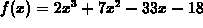 and asked to find the values of x where the first
derivative is zero or the second deriviative is zero. The following
Maple commands show a perfectly acceptable way to do this.
and asked to find the values of x where the first
derivative is zero or the second deriviative is zero. The following
Maple commands show a perfectly acceptable way to do this.
> poly := 2*x^3+7*x^2-33*x-18;

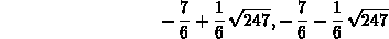
> solve(diff(poly,x)=0,x);

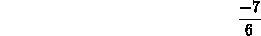
> solve(diff(poly,x,x)=0,x);

You could, of course define the polynomial to be a function as in the following example.
> f := x -> 2*x^3+7*x^2-33*x-18;

> solve(diff(f(x),x)=0,x);
> solve(diff(f(x),x,x)=0,x);
On the other hand, it is certainly not necessary in
solving the above problem to define the first and second derivatives
of  as Maple functions. Doing so would just add more commands,
but wouldn't make what you are doing any easier or clearer.
as Maple functions. Doing so would just add more commands,
but wouldn't make what you are doing any easier or clearer.
Another situation where functions can make your work easier to carry
out is when you have functions depending on parameters and you want to
explore the effect the parameter has on the function. For example
suppose you wanted to study the effect of the parameter v on the
behavior of the function 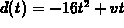 , which arises in studying
the motion of particles in one dimension. Here the parameter v can
be thought of as the initial velocity of the particle. If you define
d in Maple as a function of both t and v with the following
command
, which arises in studying
the motion of particles in one dimension. Here the parameter v can
be thought of as the initial velocity of the particle. If you define
d in Maple as a function of both t and v with the following
command
> d := (t,v) -> -16*t^2+v*t;

then it is very easy to do things like the following.
The following commands demonstrate these three points.
> d(t,5);

> plot(d(t,5),d(t,10),d(t,15),t=0..1);
> plot3d(d(t,v),t=0..2,v=0..20);
If you defined d to just be a function of t, then you could do the first and second tasks with the following commands.
> d2 := t -> -16*t^2+v*t;

> v := 5;

> d2(t);

> plot(subs(v=5,d2(t)),subs(v=10,d2(t)),subs(v=15,d2(t)),t=0..1);
However, since we set the value of v to be 5, it is a little surprising that the last command works. It turns out that the reason it works is due to Maple's evaluation rules, which can be a little commplicated and are a major source of problems in Maple programming.
The fact that we set the value of v catches up with us when we attempt to do the third task, as shown below.
> plot3d(d2(t),t=0..2,v=0..20);
Error, (in plot3d) bad range arguments, t = 0 .. 2, 5 = 0 .. 20
This example actually illustrates two points. The first is that it is simpler and more elegant to define functions than to use the subs command. The second point is that it is not a good idea to assign fixed values to variables that you are going to want to treat as parameters, as we did with v above.
If you find yourself in this situation, there is a simple way to make a variable whose value has been assigned back into a free variable. Just use an assignment statement like the following.
> v := 'v';
