The SAS data set SASDATA.STATOPOLIS contains information on 100,000 households.1 For the purposes of this lab, these 100,000 households will constitute the population.
- A.
- Open SASDATA.STATOPOLIS in SAS/INSIGHT now
(Recall that to get into SAS/INSIGHT you choose Solutions: Analysis: Interactive Data Analysis from
any of the main SAS windows). You will see that there
are four variables in the data set:
- o
- HHSIZE: household size.
- o
- VALUEH: the value of the house.
- o
- H_INCOME: household income.
- o
- H_GENDER: gender of the head of the household (0=female, 1=male)
- B.
- Do a distribution analysis on HHSIZE (by choosing
Analyze: Distribution ( Y )). You will want to
change the intervals for the density histogram. To
do this,
- 1.
- Click on the little triangle at the
lower left of the box containing the histogram, and then on ``Ticks.''
- 2.
- Set the First Tick to .5, the Last
Tick to 8.5, the Tick Increment
to 1, the Axis Minimum to 0, and the Axis Maximum to 9.
The density histogram that results is the population histogram: there is one bar for each value of HHSIZE in the population, and the area of the bar is the proportion of the population that takes that value. Clicking on a bar will display its height, which here equals its area, since the intervals are 1 unit wide. (For instance the height/area of the bar for HHSIZE=5 is 0.0971). By holding down the control key and clicking on each bar in turn, the histogram will display the heights of all bars. Do this now, then print or save the histogram for later use in this lab and for your lab report.2
Leave this distribution analysis window open (you will be returning to it later) and go to C.
- C.
- Do a distribution analysis on H_INCOME.
Notice that the density histogram has many bars, in
contrast to the density histogram you produced for
HHSIZE. This is because HHSIZE is discrete, taking
only eight values. H_INCOME takes so many different
values, it is easier to model its distribution using a
density curve. To see what such a curve might look
like, select Curves: Kernel Density then click
OK. Print or save this histogram with the
density curve for your lab report.
It may seem surprising, but even experts do not all agree on a single meaning of probability. We will focus on the two meanings that are most often used. These are probability as a population proportion, and probability as a long run proportion.
- A.
- Probability As A Population
Proportion.
We will consider the discrete and continuous cases separately.
- 1.
- The Discrete Case.
Consider again the STATOPOLIS population. How can we define the probability that a household has five members? One meaningful way is to define it as the proportion of all five member households in the population. In the STATOPOLIS population, 9,711 of the 100,000 households have five members, so the probability that a household has five members is
 .
.
In Part I.B. you calculated the height/area of each bar in the HHSIZE density histogram. These numbers are population proportions of households of each size. A check of the histogram you produced should show its height/area to be 0.09711.
The probabilities that a household has 1, 2, 3, 4, 6, 7, and 8 members summarize the pattern of variation of household size in the population. This summary is called the distribution model of HHSIZE. In your lab report, indicate the interpretation of these probabilities as population proportions.
- 2.
- The Continuous Case.
Consider again the H_INCOME population. Its distribution model is called a gamma distribution model with parameters
 and
and
 . The density curve for
this gamma distribution is
. The density curve for
this gamma distribution is
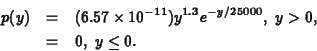
The gamma distribution is common in probability and statistics, and probabilities involving it may be computed using the SAS macro NPROBS. Access this macro now and use it to compute the proportion of household incomes that, according to the model, lie between $15,000 and $50,000.3 In your lab report, indicate the interpretation of this probability as a population proportion.
- B.
- Probability As A Long Run
Proportion.
Probability can also be interpreted as the limit of proportions in random samples taken from the population. To see how this works for the STATOPOLIS data, take random samples of sizes 50, 500 and 5000 by running the SAS macro LAB4_5. The samples will be written to the SAS data files SAMP50, SAMP500, and SAMP5000 in the WORK library. Open each now in SAS/INSIGHT.
- 1.
- The Discrete Case.
Invoke a distribution analysis of HHSIZE, and alter the density histogram exactly as you did the population histogram in Part I.B. For each data set, click on the bars of the density histogram to calculate the proportion of HHSIZE values taking on each of the values 1 to 8. You will want to save or print each histogram. In your lab report, compare these proportions with the population values you computed in Part I.B. Do the sample values seem to be converging to the population values?
- 2.
- The Continuous Case
Now do the same with the proportion of H_INCOME values between 15000 and 50000. A good way to get these proportions for the three data sets is the following:
- (a)
- From the SAS/INSIGHT data sheet,
select Edit: Variables: Other.
In the resulting dialog box, select
H_INCOME as the Y variable,
 as the transformation,
15000 as
as the transformation,
15000 as  and 50000 as
  .
.
- (b)
- The above creates a variable
in the SAS/INSIGHT data sheet that
takes the value 1 if H_INCOME is
between $15,000 and $50,000, and
the value 0 otherwise. The mean of
this variable equals the proportion
of households in the sample with
incomes between $15,000 and $50,000
(can you see why?).
In your lab report, be sure to include the following:

- The histograms from I.B. and C.
- The interpretations of probabilities as
population proportions in II.A.1.
- Calculation of probability and its
interpretation as a population proportion in II.A.2.
- Proportions of data values in SAMP50,
500 and 5000 taking on specified values,
comparisons with population values, and conclusions
regarding convergence (see II.B.)