The SAS data set SASDATA.STATOPOLIS contains information on 100,000 households.1For the purposes of this lab, these 100,000 households will constitute the population.
- A.
- Open SASDATA.STATOPOLIS in SAS/INSIGHT now (Recall that
to get into SAS/INSIGHT you choose Solutions: Analysis: Interactive Data
Analysis from any of the main SAS windows). You
will see that there are four variables in the data set:
- o
- HHSIZE: household size.
- o
- VALUEH: the value of the house.
- o
- H_INCOME: household income.
- o
- H_GENDER: gender of the head of the household (0=female, 1=male)
- B.
- Do a distribution analysis on H_INCOME (by
choosing Analyze: Distribution ( Y )).
Notice that the density histogram has many bars. H_INCOME takes so many different values, it is easier to model its distribution using a density curve. To see what such a curve might look like, select Curves: Kernel Density then click OK. Print or save this histogram with the density curve for your lab report.
By using some statistical trickery, we have managed to come up with a standard density curve that models the population closely. It's called a gamma distribution with parameters
 and
and
 . The density curve for this gamma
distribution is
. The density curve for this gamma
distribution is
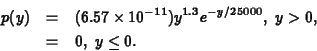
The gamma distribution is common in probability and statistics, and probabilities involving it may be computed using the SAS macro NPROBS, which you will do in Part II of this lab. In the rest of the lab, we will assume this gamma distribution is the population distribution.
In this part of the lab, you will take three random samples from the population: one of size 5, one of size 50, and one of size 2. You will use the data in the size 5 and size 50 samples to (1) estimate the population mean household income using a confidence interval, (2) predict a new household income drawn from the population using a prediction interval, and (3) obtain a range of values that with high probability contains at least 95% of all household incomes in the population using a tolerance interval. You will use the sample of size 2 to check whether the prediction intervals you computed for sample sizes 5 and 50 contain a new observation from the population.
After computing these quantities on the data you sampled, you will pool your results with those of others in the class. This pooled data will be used in this lab next term to evaluate the performance of the three kinds of intervals Since this is a new lab, we have created a pooled data set (under the name SASDATA.LAB5_3) for you to analyze in Part III of this lab.
- A.
- Select the samples by running the SAS macro
LAB5_3.2 The samples
of size 5, 50 and 2 will be written to the SAS data sets
WORK.SAMP5, WORK.SAMP50, and WORK.NEWOBS,
respectively.
- B.
- Open each of the samples in SAS/INSIGHT. For
the samples of size 5 and 50,
- 1.
- Compute the mean,
 , and a 95%
confidence interval for the population mean
, and a 95%
confidence interval for the population mean
 . To do this, choose Analyze:
Distribution( Y ) and input H_INCOME as the the
Y variable. From the resulting analysis window,
select Tables: Basic Confidence Intervals:
95%. The first row of the 95% Confidence
Intervals table contains (under
Estimate) and the confidence interval endpoints (LCL
and UCL). Now evaluate whether this interval
contains the true population mean . Write
down these four quantities for both the SAMP5 and
SAMP50 data sets.
. To do this, choose Analyze:
Distribution( Y ) and input H_INCOME as the the
Y variable. From the resulting analysis window,
select Tables: Basic Confidence Intervals:
95%. The first row of the 95% Confidence
Intervals table contains (under
Estimate) and the confidence interval endpoints (LCL
and UCL). Now evaluate whether this interval
contains the true population mean . Write
down these four quantities for both the SAMP5 and
SAMP50 data sets.
- 2.
- For each sample, compute a level 0.95
prediction interval for a new observation. To do
this, obtain the sample mean, , the
sample variance,
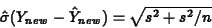
 , and the square of the
standard error of the mean,
, and the square of the
standard error of the mean,  . The first two
are found in the Moments table in the SAS: Distribution window. The second is obtained
by squaring the quantity labelled Std Mean in
that table. Use the and values to
compute the estimated standard error of prediction
using the formula
. The first two
are found in the Moments table in the SAS: Distribution window. The second is obtained
by squaring the quantity labelled Std Mean in
that table. Use the and values to
compute the estimated standard error of prediction
using the formula
Now compute the prediction interval using the formula
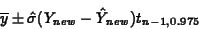
After you obtain the first prediction interval, check whether it contains the first observation in the data set WORK.NEWOBS. After you obtain the second prediction interval, check whether it contains the second observation in the data set WORK.NEWOBS. For both the SAMP5 and SAMP50 data sets, write down the prediction interval, the corresponding new observation from WORK.NEWOBS, and whether the prediction interval contains that new observation.
- 3.
- For the samples of size 5 and 50, compute a
normal theory level 0.95 tolerance interval for a
proportion 0.99 of the population values. Use
formula (5.27), p. 269 of the text, or you can use
the SAS macro NORTOL.
Once you have obtained the tolerance interval, check whether it really contains at least 99% of all population household incomes. To do this, use the SAS macro NPROBS. The following illustrates how:
Suppose the tolerance interval you obtained has endpoints 5,000 and 190,000. Access the macros by selecting Solutions: EIS/OLAP Application Builder: Applications: Run Private Applications. Select the macro NPROBS. In the macro window, choose the gamma distribution with parameters
and , and interval endpoints  and
and  . The resulting value is 0.9849,
meaning that 98.49% of all household incomes lie
between $5000 and $190000. therefore, this
tolerance interval fails to contain at least 99% of
all household incomes in the
population.3
. The resulting value is 0.9849,
meaning that 98.49% of all household incomes lie
between $5000 and $190000. therefore, this
tolerance interval fails to contain at least 99% of
all household incomes in the
population.3
For each of the data sets your group generates, write down the tolerance interval, the proportion of the population values it contains, and whether it contains at least 99% of all household incomes in the population.
- 4.
- When you have completed parts 1-3 above for
each sample, submit the results to the TA. The
values for the entire class will be input to a SAS
data set for use next term. Because this is a new
lab, we have created a data set of 100 observations
for you. You will find it in the SAS data set
SASDATA.LAB5_3.
- III.
- Analysis
Open the SAS data set SASDATA.LAB5_3 in SAS/INSIGHT now (Recall that to get into SAS/INSIGHT you choose Solutions: Analysis: Interactive Data Analysis from any of the main SAS windows). The data set has the following variables:
- o
- LCL5: The lower confidence limit from the
sample of size 5.
- o
- UCL5: The upper confidence limit from the
sample of size 5.
- o
- INCL5: 1 if the confidence interval from the
sample of size 5 includes the population mean; 0
otherwise.
- o
- LCL50: The lower confidence limit from the
sample of size 50.
- o
- UCL50: The upper confidence limit from the
sample of size 50.
- o
- INCL50: 1 if the confidence interval from the
sample of size 50 includes the population mean; 0
otherwise.
- o
- LPL5: The lower prediction limit from the
sample of size 5.
- o
- UPL5: The upper prediction limit from the
sample of size 5.
- o
- NEW5: The new observation corresponding to
the sample giving the prediction interval from the
sample of size 5.
- o
- INPL5: 1 if the prediction interval from the
sample of size 5 includes the corresponding new
observation; 0 otherwise.
- o
- LPL50: The lower prediction limit from the
sample of size 50.
- o
- UPL50: The upper prediction limit from the
sample of size 50.
- o
- NEW50: The new observation corresponding to
the sample giving the prediction interval from the
sample of size 50.
- o
- INPL50: 1 if the prediction interval from the
sample of size 50 includes the corresponding new
observation; 0 otherwise.
- o
- LTOL5: The lower tolerance limit from the
sample of size 5.
- o
- UTOL5: The upper tolerance limit from the
sample of size 5.
- o
- PROP5: The proportion of population values
covered by the tolerance interval from the
sample of size 5.
- o
- INTOL5: 1 if the tolerance interval from the
sample of size 5 includes at least 99% of the
population values; 0 otherwise.
- o
- LTOL50: The lower tolerance limit from the
sample of size 50.
- o
- UTOL50: The upper tolerance limit from the
sample of size 50.
- o
- PROP50: The proportion of population values
covered by the tolerance interval from the
sample of size 50.
- o
- INTOL50: 1 if the tolerance interval from
the sample of size 50 includes at least 99% of the
population values; 0 otherwise.
Have a look at these to familiarize yourself with them.
- A.
- Run the SAS Macro LAB5_3CI. This will
produce two plots of the confidence intervals in
the SASDATA.LAB5_3 data set: one for sample size 5
and the other for sample size 50. The plots are
color-coded: green indicates the population mean,
 is contained in the interval, and red
indicates it is not. The macro also computes the
mean width of the confidence intervals. Print the
plots and write down the values of the mean widths
for submission with your lab report.
is contained in the interval, and red
indicates it is not. The macro also computes the
mean width of the confidence intervals. Print the
plots and write down the values of the mean widths
for submission with your lab report.
Two issues in the performance of confidence intervals are coverage and precision.
- 1.
- Coverage refers to the proportion of
intervals that contain the true parameter
value. Calculate the coverage from the
confidence interval plots for sample sizes
5 and 50 for submission with your lab
report. Are they both close to the nominal
coverage of 0.95? To each other?
- 2.
- Precision refers to interval width.
Compare the mean interval widths for both
sample sizes. Theory says that the width
should be proportional to
 (since the standard error of the mean is
 ). Is this the case here?
Justify your answer.
). Is this the case here?
Justify your answer.
- B.
- Run the SAS Macro LAB5_3PI. This will
produce two plots of the prediction intervals in
the SASDATA.LAB5_3 data set: one for sample size 5
and the other for sample size 50. The plots are
color-coded: green indicates the appropriate new
observation (NEW5 or NEW50) is contained in the
interval, and red indicates it is not. The macro
also computes the mean width of the prediction
intervals. Print the plots and write down the
values of the mean widths for submission with your
lab report.
The two issues of coverage and precision are also important for the analysis of prediction intervals.
- 1.
- For prediction intervals, coverage
refers to the proportion of intervals that
contain their corresponding new
observation. Calculate the coverage from
the confidence interval plots for sample
sizes 5 and 50 for submission with your lab
report. Are they both close to the nominal
coverage of 0.95? To each other?
- 2.
- As it does for confidence intervals,
precision of prediction intervals refers to
interval width. Compare the mean interval
widths for both sample sizes. Theory says
that the width should be proportional to
 (since the standard error of
the prediction error is
(since the standard error of
the prediction error is
 ). Is this the case
here? Justify your answer.
). Is this the case
here? Justify your answer.
- C.
- Run the SAS Macro L5_3TI5. This will
produce a plot of the tolerance intervals in the
SASDATA.LAB5_3 data set based on the samples of
size 5. The plot has two parts: one showing the
intervals and the second showing the proportion of
population values contained within each interval.
Both parts are color coded: green indicates that
at least 99% of the population values lie between
the endpoints of the interval, and red indicates
the percentage is less than 99. The macro also
computes the mean width of the tolerance
intervals. Print the plot and write down the
values of the mean widths for submission with your
lab report.
- D.
- Run the SAS Macro L5_3TI50. This macro
produces the same output as L5_3TI5, but for
samples of size 50. Print the plot and write down
the values of the mean widths for submission with
your lab report.
The two issues of coverage and precision are also important for the analysis of tolerance intervals.
- 1.
- For prediction intervals, coverage means
that the interval contains at least the
desired proportion of population values
(here the proportion is 0.99). Calculate the
coverage from the confidence interval plots
for sample sizes 5 and 50 for submission
with your lab report. Are they both close to
the nominal coverage of 0.95? To each
other?
- 2.
- As it does for the other types of
intervals, precision of tolerance intervals
refers to interval width. Compare the mean
interval widths for both sample sizes.
- E.
- Based on what you have seen in parts III.
A.-D., summarize how sample size affects coverage
and precision for the three types of
intervals.
The population distribution of H_INCOME is nonnormal. In fact, it's pretty heavily right skewed. For some types of intervals this will make a large difference and for some it will make little difference. Which of the intervals you evaluated do you think might have been affected by the nonnormality of the population distribution? In what way were they affected? Explain your choices.
- IV.
- Lab Report Checklist
In your lab report, be sure to include the following:

- Histogram of population values with
density curve (I.A.).
- For the confidence intervals you
compute by hand: (1) The sample size (5 or 50) (2)
The sample mean, (3) The interval
(4) Whether it contains the population mean,
. (II.B.1.).
- For the prediction intervals you
compute by hand: (1) The sample size (5 or 50) (2)
The interval (3) The new value to be predicted
(4) Whether it contains the new value. (II.B.2.).
- For the tolerance intervals you
compute by hand: (1) The sample size (5 or 50) (2)
The interval (3) The proportion of population
values it contains (4) Whether it contains at least
99% of all population values. (II.B.3.).
- Two plots, mean widths for
confidence intervals, and coverage (III.A.).
- Two plots, mean widths for
prediction intervals, and coverage (III.B.).
- Two plots, mean widths for tolerance
intervals, and coverage (III.C. and D.).
- Overall summary of findings (III.E.).