The SAS data set SASDATA.STATOPOLIS contains information on 100,000 households.1For the purposes of this lab, these 100,000 households will constitute the population.
- A.
- Open SASDATA.STATOPOLIS in SAS/INSIGHT now
(Recall that to get into SAS/INSIGHT you choose Solutions:
Analysis: Interactive Data Analysis from any of the main SAS
windows). You will see that there are four variables in the data set:
- o
- HHSIZE: household size.
- o
- VALUEH: the value of the house.
- o
- H_INCOME: household income.
- o
- H_GENDER: gender of the head of the household (0=female, 1=male)
- B.
- Do a distribution analysis on H_INCOME (by
choosing Analyze: Distribution ( Y )).
Notice that the density histogram has many bars. H_INCOME takes so many different values, it is easier to model its distribution using a density curve. To see what such a curve might look like, select Curves: Kernel Density then click OK. Print or save this histogram with the density curve for your lab report.
By using some statistical trickery, we have managed to come up with a standard density curve that models the population closely. It's called a gamma distribution with parameters
 and
and
 . The density curve for this gamma
distribution is
. The density curve for this gamma
distribution is
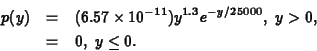
The gamma distribution is common in probability and statistics, and probabilities involving it may be computed using the SAS macro NPROBS, which you will do in Part II of this lab. In the rest of the lab, we will assume this gamma distribution is the population distribution.
In this part of the lab, you will take three random samples from the population: one of size 5, one of size 50, and one of size 2. You will use the data in the size 5 and size 50 samples to predict a new household income drawn from the population using a prediction interval. You will use the sample of size 2 to check whether the prediction intervals you computed for sample sizes 5 and 50 contain a new observation from the population.
After computing these quantities on the data you sampled, you will pool your results with those of others in the class. This pooled data will be used in this lab next term to evaluate the performance of the three kinds of intervals Since this is a new lab, we have created a pooled data set (under the name SASDATA.LAB5_3pi) for you to analyze in Part III of this lab.
- A.
- Select the samples by running the SAS macro
LAB5_3.2 The samples
of size 5, 50 and 2 will be written to the SAS data sets
WORK.SAMP5, WORK.SAMP50, and WORK.NEWOBS,
respectively.
- B.
- Open each of the samples in SAS/INSIGHT. For each
of the samples of size 5 and 50, compute a level 0.95
prediction interval for a new observation. To do this,
obtain the sample mean,
 , and the sample
standard deviation
, and the sample
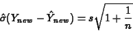
standard deviation  , which are found in the Moments table in the SAS: Distribution window. The
estimated standard error of prediction is computed using
the formula
, which are found in the Moments table in the SAS: Distribution window. The
estimated standard error of prediction is computed using
the formula
Now compute the prediction interval using the formula
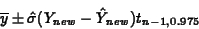
After you obtain the first prediction interval, check whether it contains the first observation in the data set WORK.NEWOBS. After you obtain the second prediction interval, check whether it contains the second observation in the data set WORK.NEWOBS. For both the SAMP5 and SAMP50 data sets, write down the prediction interval, the corresponding new observation from WORK.NEWOBS, and whether the prediction interval contains that new observation, and submit the results to the TA. The values for the entire class will be input to a SAS data set for use next term. Because this is a new lab, we have created a data set of 100 observations for you. You will find it in the SAS data set SASDATA.LAB5_3PI.
Open the SAS data set SASDATA.LAB5_3PI in SAS/INSIGHT now (Recall that to get into SAS/INSIGHT you choose Solutions: Analysis: Interactive Data Analysis from any of the main SAS windows). The data set has the following variables:
- o
- LPL5: The lower prediction limit from the
sample of size 5.
- o
- UPL5: The upper prediction limit from the
sample of size 5.
- o
- NEW5: The new observation corresponding to
the sample giving the prediction interval from the
sample of size 5.
- o
- INPL5: 1 if the prediction interval from the
sample of size 5 includes the corresponding new
observation; 0 otherwise.
- o
- LPL50: The lower prediction limit from the
sample of size 50.
- o
- UPL50: The upper prediction limit from the
sample of size 50.
- o
- NEW50: The new observation corresponding to
the sample giving the prediction interval from the
sample of size 50.
- o
- INPL50: 1 if the prediction interval from the
sample of size 50 includes the corresponding new
observation; 0 otherwise.
Have a look at these to familiarize yourself with them.
- A.
- Run the SAS Macro LAB5_3PI. This will
produce two plots of the prediction intervals in
the SASDATA.LAB5_3PI data set: one for sample size 5
and the other for sample size 50. The plots are
color-coded: green indicates the appropriate new
observation (NEW5 or NEW50) is contained in the
interval, and red indicates it is not. The macro
also computes the mean width of the prediction
intervals. Print the plots and write down the
values of the mean widths for submission with your
lab report.
Two issues in the performance of prediction intervals are coverage and precision.
- 1.
- Coverage refers to the proportion of
intervals that contain the new observation.
Calculate the coverage from the
prediction interval plots for sample sizes
5 and 50 for submission with your lab
report. Are they both close to the nominal
coverage of 0.95? To each other?
- 2.
- Precision refers to interval width.
Compare the mean interval widths for both
sample sizes. Theory says that the width
should be proportional to
 (since the standard
error of the prediction error is
(since the standard
error of the prediction error is
 ). Is this the case
here? Justify your answer.
). Is this the case
here? Justify your answer.
- B.
- Based on what you have seen in III. A.,
summarize how sample size affects coverage and
precision for the prediction intervals.
The population distribution of H_INCOME is nonnormal. In fact, it's pretty heavily right skewed. Sometimes this can have an adverse effect on the coverage of prediction intervals. Do you think the skewness affected the coverage of the prediction intervals you evaluated? Explain.
In your lab report, be sure to include the following:

- Histogram of population values with
density curve (I.B.).
- For the prediction intervals you
compute by hand: (1) The sample size (5 or 50) (2)
The sample mean, (3) The interval
(4) The new observation to be predicted (5) Whether
the interval contains the new value (II.B.).
- Two plots, mean widths for prediction
intervals and comparison with theoretical, and
coverage (III.A.).
- Overall summary of findings (III.B.).