


Next: About this document ...
Up: lab_template
Previous: lab_template
Subsections
The purpose of this lab is to locate roots and find solutions to one equation.
There are several different methods for finding the roots or the zeros of an expression. For instance, if it is possible, you could factor the expression and set each factor equal to zero. This can be done by using the Maple factor command. Another method for finding roots is to plot the expression and estimate the zeros by looking at where the graph intersects the  -axis. This is not the best method since the root is not always an integer value and therefore, it will be difficult to get the exact roots. Plotting the expression may not give us the exact roots, however it is very useful to see how many roots there actually are. The example below shows how to factor and plot the expression
 .
.
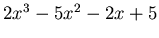
> j := 2*x^3-5*x^2-2*x+5;
> factor(j);
> plot(j,x=-100..100);
> plot(j,x=-3..3);
Note that there is only one argument that is necessary for the factor command. The plot command is used to verify that there are exactly three roots for this expression. As the two plot commands show, it is sometimes difficult to see exactly how many roots there are based on the range that is chosen. You should try different ranges until you obtain a plot that is acceptable. Here are a few more examples.
> factor(sin(x)+3);
> plot(sin(x)+3,x=-4*Pi..4*Pi);
> factor(x*sin(x)-1);
> plot(x*sin(x)-1,x=-50..50);
When an expression is already in factored form or cannot be factored, the Maple output is the same expression that was entered. Remember, not every expression has roots. That is, some expressions, when plotted, don't intersect with the -axis at all while others may intersect the -axis infinitely many times. When an expression cannot be factored, this does not necessarily imply that there are no roots. You may want to plot the expression first to see if there are any roots. The example above shows that  cannot be factored, however you can see by the plot that there are infinitely many roots.
Finding roots of an expression or a function
cannot be factored, however you can see by the plot that there are infinitely many roots.
Finding roots of an expression or a function  is the same as solving the equation
  . Since not every expression can be factored and it is sometimes difficult to get the exact root based on the plot, the best method for finding roots is to use Maple's solving capabilities. First, a plot of the function or expression is needed to determine how many roots there are. Once you know how many roots there are, you can use the Maple solve command.
The basic syntax for the solve command is
. Since not every expression can be factored and it is sometimes difficult to get the exact root based on the plot, the best method for finding roots is to use Maple's solving capabilities. First, a plot of the function or expression is needed to determine how many roots there are. Once you know how many roots there are, you can use the Maple solve command.
The basic syntax for the solve command is
> solve(equation,variable);
The following example illustrates how we can find the roots of the function
 using the solve command.
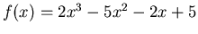
> f := x-> 2*x^3-5*x^2-2*x+5;
> solve(f(x)=0,x);
> solve(2*x^3-5*x^2-2*x+5=0,x);
Here the ``='' sign is used in the equation, not ``:='' which is used for assignment. If you forget to type in an equation and only type in an expression without setting it equal to zero, Maple automatically sets the expression equal to zero. The solve command is not only used for solving for zeros, it can be used to solve other equations as well. In the examples below, you can see some of the solving capabilities of Maple.
> solve(sin(x)=tan(x),x);
> solve(x^2+2*x-1=x^2+1,x);
Unfortunately, many equations cannot be solved analytically. For example, we can use the quadratic formula to find the roots of any quadratic polynomial. There also exist formulas for finding roots of cubic and quartic (fourth order) equations, but they are so complicated that they are hardly ever used. However, it can be proven that there is no general formula for the roots of a fifth or higher order polynomial. Once we get away from polynomial equations, the situation is even worse. For example, even the relatively simple equation sin(x) = x/2 has no analytical solution.
If an equation cannot be solved analytically, then the only possibility is to solve it numerically. In Maple, the command to use is fsolve. The syntax for fsolve is very similar to that of solve. Sometimes when the solve command is used, the output looks like:
> solve(sin(x)=x/2,x);
                       RootOf(_Z-2sin(_Z))
This is not incorrect, as some of the zeros of a function may be imaginary and others may be real. What you need to do is read the output carefully looking for real solutions (each solution is separated by a comma) or use the fsolve command instead. A simple example will show how we can find solutions to the equation
 .
.
> fsolve(sin(x) = x/2, x);
Note that the result is a decimal approximation and is not exact. Also, a plot of both equations on the same graph will show that this solution is not complete. There are two other intersection points that the fsolve command did not output. The fsolve command allows us to solve the equation in a range of values by replacing the second argument with what looks like a plot range. This method only works for the fsolve command and not for the solve command. Try the following examples to see how we can get all solutions to this equation.
> plot({sin(x),x/2},x=-2*Pi..2*Pi);
> fsolve(sin(x) = x/2, x=-3..-1);
> fsolve(sin(x) = x/2, x=-1..1);
> fsolve(sin(x) = x/2, x=1..3);
Once you have solved an equation, you may want to use the output or the solution later. In order to label the output to a solution, you need to assign a label in the same line as the solve or fsolve command. For example,
> expr2 := x^2 + 2*x - 5;
> answer := solve(expr2=0,x);
> evalf(subs(x=answer[1], expr2));
Here, an expression was defined first and then the solution was assigned to the label ``answer''. Note that there was more than one solution. In order to substitute the answer that was listed first back into the expression, the subs command was used and [1] was added onto the variable name answer to distinguish the first solution from the second.
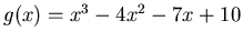
- Given the expression
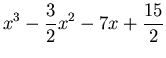 ,
,
- Plot the expression and state how many roots there are.
- Use the Maple factor command to factor the expression.
- Use the Maple solve command to find roots of the expression.
- Use the Maple fsolve command to find roots of the expression.
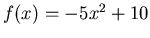
- Given the function
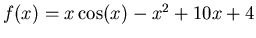 ,
,
- Plot the function over the interval
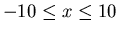 .
.
- Find all roots using the fsolve command and label the output.
- Substitute each root back into the function to show that the answer is zero.
- Find all points where the functions
 and
and
 intersect each other. A plot of both functions on the same graph may be necessary to ensure that you have found all intersection points. Once you have found the coordinate(s), substitute the solution(s) back into either function to get the corresponding
  coordinate(s).
Next: About this document ...
Up: lab_template
Previous: lab_template
Dina Solitro
2004-09-13