Subsections

• Linear Approximation
• Newton's Method
• Exercises

Linear Approximation and Newton's Method

Linear Approximation

Suppose that $f(x)$ is a differentiable function and that $a$ is some fixed number in the domain of $f$. We define the linear approximation to $f(x)$ at $x = a, f_{T}(x,a)$ by the equation

$$f_{T}(x,a) = f'(a)(x-a)+f(a).$$

In this equation, the parameter $a$ is called the base point, and $x$ is the independent variable. You may recognize the equation as the equation of the tangent line at the point $a$. It is this line that will be used to make the linear approximation. For example if $f(x) = x^2$, then $f_{T}(x,1)$ would be the line tangent to the parabola at $x = 1$

> f:=x->x^2;
> fT1:=D(f)(1)*(x-1)+f(1);
> plot({f(x),fT1},x=-1..3);

Obviously the two things the function and the tangentline have in common at $x = a$ are their y-value and their slope. Looking at the plot, the line will approximate the function exactly at the base point a and the approximation will be close if you stay close to that base point. To see how far off the approximation becomes on the given interval of the plot it is easy to see that the largest errors occur at the ends of the interval, i.e. $x = -1$ and $x = 3$. Simply subtract the y-values to calculate the error.

> abs(f(-1)-subs(x=-1,fT1));
> abs(f(3)-subs(x=3,fT1));

Notice that the error grows to four at each end of the interval. How could you find an interval such that the greatest error will be a specific value? Think about this as it will appear in the exercises.

Newton's Method

Many problems in mathematics, science, engineering, and business eventually come down to finding the roots of a nonlinear equation. It is a sad fact of life that many mathematical equations cannot be solved analytically. You already know about the formula for solving quadratic polynomial equations. You might not know, however, that there are formulas for solving cubic and quartic polynomial equations. Unfortunately, these formulas are so cumbersome that they are hardly ever used. Even more unfortunately, it has been proven that no formula can exist for finding roots of quintic or higher polynomials. Furthermore, if your equations involve trig functions, then it is even easier to find equations that do not have analytical solutions. For example, the following simple equation cannot be solved to give a formula for x.

$$\sin(x)=\frac{x}{2}$$

The need to solve nonlinear equations that cannot be solved analytically has led to the development of numerical methods. One of the most commonly used numerical methods is called Newton's method or the Newton-Raphson method. The idea of Newton's method is relatively simple. Suppose you have a nonlinear equation of the form

$$f(x)=0$$

where $f$ is a differentiable function. Then the idea of Newton's method is to start with an initial guess $$x_0$$ for the root and to use the tangent line to $f$ at $$x=x0$$ to approximate $f$. The equation for the tangent line appears below.

$$y =f(x_0)+f'(x_0)(x-x_0)$$

If the tangent line is a good approximation to $f$, then the $x$ intercept of the tangent line should be a good approximation to the root. Call this value of $x$ where the tangent line intersects the $x$ axis $$x_1$$. We can solve the equation above to get the following formula.

$$x_1=x_0-\frac{f(x_0)}{f'(x_0)}$$

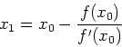
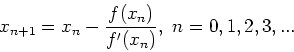
In practice, unless the starting point $$x_0$$ is very close to the root, the value $$x_1$$ is not close enough to the root we are seeking, so Newton's method is applied again using the tangent line at $$x=x_1$$. This process can be repeated, leading to a sequence of values where the value of $$x_{n+1}$$ is determined from the equation

$$x_{n+1}=x_n-\frac{f(x_n)}{f'(x_n)},~n=0,1,2,3,...$$

For example, consider the equation from above,

$$\sin(x)=\frac{x}{2}$$

If you want to solve this equation using Newton's method, the first thing to do is to write it in standard form as

$$\sin(x)-\frac{x}{2}=0$$

Then, plot the expression to get an idea of where the roots are. You may have to adjust the plot range to locate all of the roots. The following commands show that there are exactly three roots, one at $x=0$, and two others at about 2 and -2.

> f:=x->sin(x)-x/2;
> plot(f(x),x=-6..6);

It isn't very hard to write a Maple command that will do one step of Newton's method. The examples below show a very simple method for doing so, using the function $f$ defined above and a starting value of $x=2.2$. Further iterations can be obtained by using composition, as shown below

> newt:=x->x-f(x)/D(f)(x);
> newt(2.2);
> newt(newt(2.2));
> (newt@@3)(2.2);

However, to simplify things for you, two commands, Newton and NewtonPlot, have been programmed for you. The Newton command takes three arguments: the function, the starting value, and the number of iterations. See the example below for three iterations. Note that these commands are part of the CalcP7 package, so you must load the package first.

> with(CalcP7):
> Newton(f(x),x=2.2,3);
> NewtonPlot(f(x),x=2.2);

One of the problems with Newton's method is knowing when to stop. With a numerical method, you can never get a root exactly, but only a numerical approximation to the root. There are basically two measures of how good your approximation to the root is. One is the absolute value of $f(xn)$. If this number is less than a certain tolerance, then you should have a good approximation to the root. The other measure is the change in the value of $$x_n$$. If the value of

$$x_n$$ and $$x_{n+1}$$ are very close, then this can also be a criterion for stopping. You should go back to the example above and experiment with changing the number of iterations.

The worst thing about Newton's method is that it may fail to converge. The key to getting Newton's method to converge is to select a good starting value. The best way to do this is to plot the function and determine approximately where the roots are. Then, use these values to start Newton's method.

Exercises

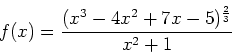
1. In your scientific studies you find that your results follow the function
   
   $$f(x) = \frac{(x^3-4x^2+7x-5)^{\frac{2}{3}}}{x^2+1}$$
   
   
   1. You want to evaluate data around the base point $x = 2$ but you don't want to work with such a messy function. What is the linear approximation to this function at this base point? Plot the function and its linear approximation over the interval $1 \leq x \leq 3$.
   2. You want to make sure that your linear approximation never is in error greater than 0.01. What is the interval of x data points that you can work with? (Use the fsolve command so you can find each interval endpoint) Plot the function and the linear approximation on the interval that you found, then plot the error bounds and the error function on the same graph over the interval you found.
2. Consider the functions $\cos(x)$ and $$\frac{x}{4}$$.
   1. Solving these two functions equal to eachother is the same as solving their difference equal to zero. Plot the difference of these two functions to see how many roots there are.
   2. Use the Newton command with the function $$f(x)=\cos(x)-\frac{x}{4}$$ and the starting value $x=-0.1$. When Newton's method is used with this initial condition, what value of $n$ is required to guarantee that $$\vert f(x_k)\vert<10^{-7}$$ for all $k \geq n$? Do not exceed a value of $n=300$. Which root did you find? Once you find the $n$ that is needed and the root that is found from this $n$, delete the result from the worksheet by clicking on the bracket to the left and choose delete paragraph from the edit menu. This is to avoid a very long printout.
   3. Use a different starting values to approximate the positive root of this function and state how many interations were needed to guarantee that $$\vert f(x_k)\vert<10^{-7}$$ for all $k \geq n$.