Subsections

• Purpose
• Background
  • Exponential growth
  • Exponential Decay
  • Newton's law of cooling
  • Effective medicine dosage
  
  
• Maple commands
• Exercises

Applications of exponential and logarithmic functions

Purpose

The purpose of this lab is to use Maple to study applications of exponential and logarithmic functions. These are used to model many types of growth and decay, for example bacterial growth and radiaoctive decay. This lab also describes applications of exponential and logarithmic functions for heating and cooling and to medicine dosage

Background

Exponential growth

The simple model for growth is exponential growth, where it is assumed that $y'(t)$ is proportional to $y$. That is,

$$\frac{dy}{dt} = ky\quad\hbox{where $k$\ is a positive constant.}$$

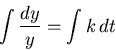
Separating the variables and integrating (see section 4.4 of the text), we have

$$\int\frac{dy}{y} = \int k\,dt$$

so that

$$\ln \mid y \mid = kt + C$$

In the case of exponential growth, we can drop the absolute value signs around $y$, because $y$ will always be a positive quantity. Solving for $y$, we obtain

$$\mid y \mid = e^{kt + C}$$

which we may write in the form $y = Ae^{kt}$, where $A$ is an arbitrary positive constant.

Exponential Decay

In a sample of a radioactive material, the rate at which atoms decay is proportional to the amount of material present. That is,

$$\frac{dA}{dt} = -kA$$

where $k>0$ is a constant. This is the same equation as in exponential growth, except that $-k$ replaces $k$. The solution is

$$A(t) = A_0 e^{-kt}$$

where $A_0$ is a positive constant. Physically, $A_0$ is the amount of material present at $t=0$.

Radioactivity is often expressed in terms of an element's half-life. For example, the half-life of carbon-14 is 5730 years. This statement means that for any given sample of ${}^{14}\hbox{C}$, after 5730 years, half of it will have undergone decay. So, if the half-life is of an element Z is $c$ years, it must be that $e^{-kc}=\frac{1}{2}$, so that $kc=\ln 2$ and $k=\frac{\ln 2}{c}$.

Newton's law of cooling

What is usually called Newton's law of cooling is a simple model for the change in temperature of an object that is in contact with an environment at a different temperature. It says that the rate of change of the temperature of an object is proportional to the difference between the object's temperature and the temperature of the environment. Mathematically, this can be expressed as the differential equation

$$\frac{dT}{dt} = -k \left( T-T_{\mathrm{out}} \right)$$

where $k$ is the constant of proportionality and $T_{\mathrm{out}}$ is the temperature of the environment. Using a technique called separation of variables it isn't hard to derive the solution

$$T(t) = T_{\mathrm{out}} + \left( T_0 - T_{\mathrm{out}} \right) e^{-kt}$$

where $T_0$ is the temperature of the object at $t=0$.

Effective medicine dosage

If a drug is administered to a patient intravenously, the concentration jumps to its highest level almost immediately. The concentration subsequently decays exponentially. If we use $C(t)$ to represent the concentration at time t, and $C_0$ to represent the concentration just after the dose is administered then our exponential decay model would be given by

$$C(t) = C_0 e^{-kt}$$

A problem facing physicians is the fact that for most drugs, there is a concentration, $m$, below which the drug is ineffective and a concentration, $M$, above which the drug is dangerous. Thus the physician would like the have the concentration $C(t)$ satisfy

$$m < C(t) < M$$

This means that the initial dose must not produce a concentration larger than $M$ and that another dose will have to be administered before the concentration reaches $m$.

Maple commands

The main functions you need are the natural exponential and natural logarithm. The Maple commands for these functions are exp and ln. Here are a few examples.

> f := x -> exp(-2*x);
> simplify(ln(3)+ln(9));
> ln(exp(x));
> simplify(ln(exp(x)),assume=real);

The assume=real is needed in the command above, because Maple usually works with complex variables. The command for base 10 logarithms is log10. Here are some examples. Note how Maple likes to convert base 10 logarithms to natural logarithms.

> log10(100);
> simplify(log10(100));
> simplify(log10(a)-log10(b),assume=real);

Sometimes you need to use experimental data to determine the value of constants in models. For example, suppose that for a particular drug, the following data were obtained. Just after the drug is injected, the concentration is 1.5 mg/ml (milligrams per milliliter). After four hours the concentration has dropped to 0.25 mg/ml. From this data we can determine values of $C_0$ and $k$ as follows. The value of $C_0$ is the initial concentration, so we have

$$C_0 = 1.5$$

To find the value of $k$ we need to solve the equation

$$0.25 = 1.5 e^{-4k}$$

which we get by plugging in $t=4$ and using the data $C(4)=0.25$. Maple commands for solving for $k$ and defining and plotting the function $C(t)$ are shown below.

> k1 := solve(0.25=1.5*exp(-4*k),k);
> C1 := t -> 1.5*exp(-k1*t);
> plot(C1(t),t=0..6);

Exercises

1. In 1935 Charles F. Richter of Cal Tech developed a scale for measuring the magnitude of earthquakes. The Richter Scale formula is given by
   
   $$M = \log_{10}(\frac{x}{c})$$
   
   
   where $M$ is the magnitude of the earthquake, $x$ is the amplitude of the largest seismic wave as measured on a standard seismograph 100 kilometers from the epicenter and $c$ is the amplitude of a reference earthquake of amplitude 1 micron on a standard seismograph at the same distance from the epicenter.
   1. When the amplitude of an earthquake is tripled, by how much does the magnitude increase?

   2. In 1989, the San Francisco Bay area suffered severe damage from an earthquake of magnitude 7.1. However, the damage was not nearly as extensive as that caused by the great quake of 1906, which has been estimated to have had magnitude 8.3. What is the ratio of the amplitude of the 1906 quake to the 1989 quake?

   3. The largest earthquake magnitude ever measured was 8.9 for an earthquake in Japan in 1933. Determine the ratio of the amplitude of this earthquake to that of the 1906 San Francisco earthquake.

2. A turkey is cooking in an oven which is at a baking temperature of $400 \, ^{\circ} \mathrm{F}$. The turkey starts at a temperature of $70 \, ^{\circ} \mathrm{F}$ and after a half hour has warmed to $90 \, ^{\circ} \mathrm{F}$. How long will it take to warm to a well-done temperature of $180 \, ^{\circ} \mathrm{F}$ ?

3. Suppose that for a certain drug, the following results were obtained. Immediately after the drug was administered, the concentration was 6.2 mg/ml. Four hours later, the concentration had dropped to 3.75 mg/ml. Determine the value of $k$ for this drug. What will the concentration be after 7 hours?