Next: About this document ...
Up: lab_template
Previous: lab_template
Subsections
There are two main ways to think of the definite integral. The easiest
one to understand is as a means for
computing areas (and volumes). The second way the definite integral is
used is as a sum. That is, we use the definite integral to ``add
things up''. Here are some examples.
- Computing net or total distance traveled by a moving object.
- Computing average values, e.g. centroids and centers of mass,
moments of inertia, and averages of probability distributions.
This lab is intended to introuduce you to Maple commands for computing
integrals, including applications of integrals.
The basic Maple command for computing definite and indefinite
integrals is the int command.
To compute the indefinite integral
with Maple:
> int(x^2,x);
Note that Maple does not include a constant of integration.
Suppose you wanted to compute the following definite
integral with Maple.
The command to use is:
> int(x^2,x=0..4);
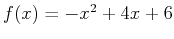
If you want to find the area bounded by the graph of two functions, you should first plot both functions on the same graph. You can then find the intersection points using either the solve or fsolve command. Once this is done, you can calculate the definite integral in Maple. An example below illustrates how this can be done in Maple by finding the area bounded by the graphs of
 and
and 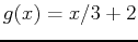 :
:
> f := x-> -x^2+4*x+6;
> g := x-> x/3+2;
> plot({f(x),g(x)},x=-2..6);
> a := fsolve(f(x)=g(x),x=-2..0);
> b := fsolve(f(x)=g(x),x=4..6);
> int(f(x)-g(x),x=a..b);
In designing mechanisms or structures, one often has to deal with
distributed forces, that is, forces that do not act at a discrete,
finite set of points. The most common example of a distributed force
is the force of gravity, which acts on all parts of any body of
matter. Other examples are pressure in fluids and electrostatic
forces, though there are many others.
One of the basic useful principles of analyzing distributed forces is
the idea of replacing them with a single, aggregate force  that acts at a single point and is somehow equivalent to the original
distributed force. This may not always be possible, but this technique
has found great use in engineering and science. As a simple example,
suppose we have gravity acting on a solid plate of uniform thickness and
density, but
irregular shape. Finding the equivalent force is really the problem of
finding the point where we could exactly balance the plate. This
balance point is often called the center of mass of the body.
that acts at a single point and is somehow equivalent to the original
distributed force. This may not always be possible, but this technique
has found great use in engineering and science. As a simple example,
suppose we have gravity acting on a solid plate of uniform thickness and
density, but
irregular shape. Finding the equivalent force is really the problem of
finding the point where we could exactly balance the plate. This
balance point is often called the center of mass of the body.
For symmetric objects, the balance point is usually easy to find. For
example, the balance point of an empty see-saw is the exact center.
Similarly, the balance points for rectangles or circles are just
the geometrical centers. For non-symmetric objects, the answer is not
so clear, but it turns out that there is a fairly simple algorithm
involving integrals for determining balance points.
We begin by restricting our attention to thin plates of uniform
density. In Engineering and Science, this type of object is called a
lamina. For mathematical purposes, we assume that the lamina is
bounded by  ,
,  ,
,  , and
, and  , with
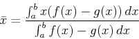
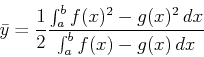
 . Then the book gives the following formulas for the coordinates
 of the center of mass.
To see where these formulas come from, we need the following
result. Suppose we have a composite body that is made up of two masses
 and
and
 and that we know the centers of mass are
 and
and
 . Then according to the principles of
mechanics, the center of mass of the composite body can be determined
from the following equations.
. Then according to the principles of
mechanics, the center of mass of the composite body can be determined
from the following equations.
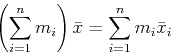
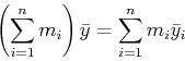
This result can be easily generalized to the case where we have a composite
body made up of  masses to give the following result.
To go from these formulas to the integral formulas presented earlier,
we first partition the interval ![$[a,b]$](img23.png) into subintervals
into subintervals
Then we approximate the lamina on each subinterval with a rectangle by
letting  be the midpoint of the
  subinterval
and using
subinterval
and using  as the top of the
rectangle and
as the top of the
rectangle and  as the bottom. This gives a rectangle of
width
as the bottom. This gives a rectangle of
width
 and height
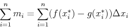
 . Assuming that the density is 1, we have the following
for the mass,
. Assuming that the density is 1, we have the following
for the mass,  , and center of mass,
 of
the rectangle.
of
the rectangle.
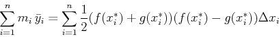
Using these relations, we get the following equations.
The right hand sides of these equations should be easy to recognize as
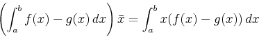
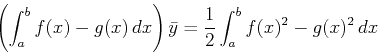
Riemann sums, so that when we take limits as goes to infinity, we
get the following in our equations for the center of mass of our
lamina.
These are easy to rearrange into the equations given in the text.
We end this section with an example, including Maple commands, for
computing the center of mass. Suppose you have a lamina bounded by the
curves
,
 whose area was computed
above and you want to compute the center of mass.
If you are not sure about the relative positions of the two curves, it
is a good idea to plot them both. Assuming constant density
whose area was computed
above and you want to compute the center of mass.
If you are not sure about the relative positions of the two curves, it
is a good idea to plot them both. Assuming constant density
 , then area and mass would be equivalent.
> plot([f(x),g(x)],x=-5..5);
> mass:=int(f(x)-g(x),x=a..b);
Now we are ready to compute the center of mass. Using labels can help you
organize your calculations and avoid mistakes.
Computing the mass separately as shown above lets you check it. If you
get a negative value for the mass, something is wrong and you have to
check what you have done. A common mistake is reversing the order of
the functions.
> xbar := int(x*(f(x)-g(x)),x=a..b)/mass;
> ybar := 1/2*int(f(x)^2-g(x)^2,x=a..b)/mass;
> plot([f(x),g(x),[[xbar,ybar]]],x=a..b,style=[line,line,point],color=black);
The plot of both functions on the same graph along with the point helps to confirm that your point is in the physical center of the lamina.
- Use Maple to compute the each of the following definite integrals:
- A)
-
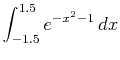 (Note the syntax for the
  function is
  .)
.)
- B)
-
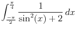 (Note: to square a trig function put the
 ^2 after the angle in parentheses)
- Find the area of the region bounded by the curves
 and
and
 .
.
- Find the coordinates of the center of mass of the lamina bounded by the curves
 and
and
 . Plot both functions on the same graph along with the point
to see if your answer makes sense.
. Plot both functions on the same graph along with the point
to see if your answer makes sense.
- Find the coordinates of the center of mass of the lamina bounded by the curves
 and
and
 . Plot both functions on the same graph along with the point
to see if your answer makes sense.
. Plot both functions on the same graph along with the point
to see if your answer makes sense.
- Find the coordinates of the center of mass of the lamina bounded by the curves
 and
and
 . Plot both functions on the same graph along with the point
to see if your answer makes sense.
. Plot both functions on the same graph along with the point
to see if your answer makes sense.
- Find the coordinates of the center of mass of the lamina bounded by the curves
 and
and  . Plot both functions on the same graph along with the point
to see if your answer makes sense.
. Plot both functions on the same graph along with the point
to see if your answer makes sense.
Next: About this document ...
Up: lab_template
Previous: lab_template
Dina J. Solitro-Rassias
2014-09-25