


Next: About this document ...
Up: lab_template
Previous: lab_template
Subsections
There are two main ways to think of the definite integral. The easiest
one to understand is as a means for
computing areas (and volumes). The second way the definite integral is
used is as a sum. That is, we use the definite integral to ``add
things up''. Here are some examples.
- Computing net or total distance traveled by a moving object.
- Computing average values, e.g. centroids and centers of mass,
moments of inertia, and averages of probability distributions.
This lab is intended to introuduce you to Maple commands for computing
integrals, including applications of integrals.
The basic Maple command for computing definite and indefinite
integrals is the int command.
To compute the indefinite integral
with Maple:
> int(x^2,x);
Note that Maple does not include a constant of integration.
Suppose you wanted to compute the following definite
integral with Maple.
The command to use is:
> int(x^2,x=0..4);
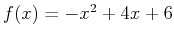
If you want to find the area bounded by the graph of two functions, you should first plot both functions on the same graph. You can then find the intersection points using either the solve or fsolve command. Once this is done, you can calculate the definite integral in Maple. An example below illustrates how this can be done in Maple by finding the area bounded by the graphs of
 and
and 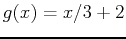 :
:
> f := x-> -x^2+4*x+6;
> g := x-> x/3+2;
> plot({f(x),g(x)},x=-2..6);
> a := fsolve(f(x)=g(x),x=-2..0);
> b := fsolve(f(x)=g(x),x=4..6);
> int(f(x)-g(x),x=a..b);
Last week, you learned about commands from Maple's student package, leftbox, rightbox, and middlebox, for plotting approximate area under a curve using left-endpoint, right-endpoint and midpoint rule.
There are also Maple commands leftsum, rightsum, and
middlesum to sum the areas of the rectangles, see the
examples below. Note the use of evalf to obtain the desired numerical
answers.
> rightsum(x^2,x=0..4,7);
> evalf(rightsum(x^2,x=0..4,7));
> evalf(leftsum(x^2,x=0..4,10));
> evalf(middlesum(x^2,x=0..4,20));
It should be clear from the graphs that adding up the areas of the
rectangles only approximates the area under the curve. However, by
increasing the number of subintervals the accuracy of the
approximation can be improved. One way to measure how good the
approximation is is the
absolute error, which is the difference between the actual answer and the
estimated answer. Later on in the course, you
will learn techniques for finding the exact answer. Approximations,
however, are important because exact answers cannot always be found.
All of the Maple commands described so far in this lab can include a third
argument to specify the number of subintervals. The default is 4
subintervals. The example below approximates the area under  from
from  to
to  using the rightsum command with 50,
100, 320 and 321 subintervals. As the number of subintervals
increases, the approximation gets closer and closer to the exact
answer. You can see this by assigning a label to the approximation,
assigning a label to the exact answer
using the rightsum command with 50,
100, 320 and 321 subintervals. As the number of subintervals
increases, the approximation gets closer and closer to the exact
answer. You can see this by assigning a label to the approximation,
assigning a label to the exact answer  and taking their
difference. The closer you are to the actual answer, the smaller the
difference. The example below shows how we can use Maple to
approximate this area with an absolute error no greater than 0.1.
and taking their
difference. The closer you are to the actual answer, the smaller the
difference. The example below shows how we can use Maple to
approximate this area with an absolute error no greater than 0.1.
\begin{verbatim}
> with(student):
> exact := 4^3/3;
> estimate := evalf(rightsum(x^2,x=0..4,321));
> evalf(abs(exact-estimate));
- The exact area under
 above the
  axis over the interval
 can be found using a definite integral. Plot
  over the given interval. Use the approximations rightsum and middlesum to determine the minimum number of subintervals required so that the estimate of this area has an error no greater than 0.001. Which method do you think is better?
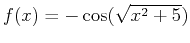
- Find the area of the region bounded by the curves
 and
and
 . Include a plot of the region bounded by the given curves.
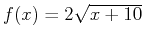
- Find the area of the region bounded by the curves
 and
and
 . Include a plot of the region bounded by the given curves.
- Find the area of the region bounded by the curves
 and
and
 . Include a plot of the region bounded by the given curves.
Next: About this document ...
Up: lab_template
Previous: lab_template
Dina J. Solitro-Rassias
2016-09-14