


Next: About this document ...
Up: lab_template
Previous: lab_template
Subsections
The purpose of this lab is to learn the basic commands needed in any Maple lab.
Expressions such as  can be entered in a similar way to variable assignment. Choose a variable name to represent the expression and assign the expression to the variable as follows.
> expr := x^3+3*x^2-x+1;
Suppose you want to enter the same expression stored in expr above, but as a function of  . In Maple, you would type
> f := x-> x^2+2*x-6;
Below is how NOT to enter a function:
> f(x) := x^2+2*x-6;
The difference between expressions and functions are first the obvious, that expressions do not have to satisfy the definition of a function in the sense that for each input , there is a unique value  . A function may be defined as an expression, but not all expressions can be defined as functions. The differences in Maple are numerous as you will see below when we evaluate the expression or function for a given value as well as when using the plot command.
In order to evaluate an expression at a given value of , you must use the subs or eval command. For example, if we wanted to evaluate the expression expr
. A function may be defined as an expression, but not all expressions can be defined as functions. The differences in Maple are numerous as you will see below when we evaluate the expression or function for a given value as well as when using the plot command.
In order to evaluate an expression at a given value of , you must use the subs or eval command. For example, if we wanted to evaluate the expression expr at
at  , the example below show how this can be done
> subs(x=2,expr);
> eval(expr,x=2);
> r:=sin(theta) + 8*theta^2;
> subs(theta=Pi/2,r);
In the subs command, the first argument tells Maple what you would like to substitute in for . The second argument tells Maple what expression you are substituting into. Note the difference in outputs when a whole number or fraction is entered compared to a decimal.
>g:=2*x/3;
>subs(x=4,g);
>eval(g,x=1/2);
>subs(x=4.0,g);
The evalf command is used when we want Maple to output the answer in decimal form.
If this command is not used, the output to your Maple commands will be calculated analytically, where as the evalf command forces Maple to calculate the answers numerically.
The evalf command has one essential argument, however a second argument can be added in order to tell how many digits we want to be in the answer as shown below.
>evalf(eval(expr,x=Pi));
>evalf(eval(expr,x=Pi),20);
In Maple, functions are much easier to evaluate than expressions. In order to evaluate the function
 at , simply type
> f(2);
You can set an expression or function equal to another expression, function, or number inside a solve command.As an example, you may want to find where the following two parabolas intersect.
> g := 9*x^2-14;
> h:=-x^2;
> plot([g,h],x=-2..2);
> solve(g=h,x);
The plot shows that there are two intersection points and the solve command finds both values.It is good to get into the habit of naming your output so you can use it in a later command. Giving the values a name makes it easy to plug them into the function to find the  values.
> ip:=solve(g=h,x);
Since there are two values called  , use [ ] to call up the one you want.
> eval(g,x=ip[1]);
> eval(h,x=ip[2]);
Therefore the two intersection points are
 and
and
 . This seems like the answer shown on the graph.
If you would like to find where the following function crosses the horizontal line
. This seems like the answer shown on the graph.
If you would like to find where the following function crosses the horizontal line  you can try the solve command.
> j:=x->2*x^3-15*x^2-2*x+5;
> k:=x->-50;
> plot([j(x),k(x)],x=-3..8);
The graph shows there should be three answers.
> solve(j(x)=k(x),x);
That is some scary output! So instead of using the algebraic solve try the numerical fsolve.
> fsolve(j(x)=k(x),x);
If you want to find where the following function crosses the x-axis, just set it equal to zero.
> f:=theta->-1/2*theta+sin(theta);
> plot(f(theta),theta=-8*Pi..8*Pi);
> solve(f(theta)=0,theta);
Wow, what is that?!?! We know from the graph that there should be three answers and solve wasn't a great option so try fsolve again.
> fsolve(f(theta)=0,theta);
Where are the other two answers!? This is actually how fsolve usually works. It shoots for one answer and only gives that one. But you can tell fsolve where to look by getting an idea from the graph and typing that domain into the fsolve command.
> a:=fsolve(f(theta)=0,theta=-5..-1);
> b:=fsolve(f(theta)=0,theta=-1..1);
> c:=fsolve(f(theta)=0,theta=1..5);
To find the values just plug in the names of the values.
> f(a);
> f(b);
> f(c);
(Of course the y-values are zero!)
Integration, the second major theme of calculus, deals with areas,
volumes, masses, and averages such as centers of mass and gyration.
In lecture you have learned that the area under a curve between two
points  and
and  can be found as a limit of a sum of areas of
rectangles which approximate the area under the curve of interest.
Not all ``area finding'' problems can be solved using analytical
techniques. The Riemann sum definition of area under a curve gives
rise to several numerical methods which can approximate the area of
interest with great accuracy.
can be found as a limit of a sum of areas of
rectangles which approximate the area under the curve of interest.
Not all ``area finding'' problems can be solved using analytical
techniques. The Riemann sum definition of area under a curve gives
rise to several numerical methods which can approximate the area of
interest with great accuracy.
Suppose is a non-negative, continuous function defined on some
interval ![$[a,b]$](img14.png) . Then by the area under the curve
. Then by the area under the curve  between
 and
and  we mean the area of the region bounded above by the
graph of , below by the -axis, on the left by the vertical
line , and on the right by the vertical line . All of the
numerical methods in this lab depend on subdividing the interval
into subintervals of uniform length.
we mean the area of the region bounded above by the
graph of , below by the -axis, on the left by the vertical
line , and on the right by the vertical line . All of the
numerical methods in this lab depend on subdividing the interval
into subintervals of uniform length.
In these simple rectangular approximation methods, the area above each
subinterval is approximated by the area of a rectangle, with the height of the
rectangle being chosen according to some rule. In particular, we will
consider the left, right and midpoint rules.
The Maple student package has commands for visualizing these
three rectangular area approximations. To use them, you first must
load the package via the with command. Then try the three commands
given below to help you understand the differences between the
three different rectangular approximations. Note that
the different rules choose rectangles which in
each case will either underestimate or overestimate the area.
> with(student):
> rightbox(x^2,x=0..4,8);
> leftbox(x^2,x=0..4,8);
> middlebox(x^2,x=0..4,8);
To commands below show how to approximate the area under the curve  using the left-endpoint rule in Maple
> f:=x->x^2;
> h:=(4-0)/8;
> h*(f(0)+f(0.5)+f(1)+f(1.5)+f(2)+f(2.5)+f(3)+f(3.5))
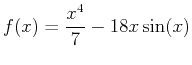
- Given the expression
 ,
,
- A)
- Plot the expression and in text state how many roots it has. That is, how many times the it crosses the x-axis.(Experiment with domain values until you find values that show the crossing points clearly.)
- B)
- Compare outputs from the Maple solve and fsolve command to find the values of where it crosses the x-axis. State the real roots in text.
- C)
- Use the Maple eval command to verify at least one of the roots to show it is zero.
- Given the functions
 and
and
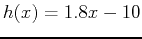
- A)
- Plot the functions. Again experiment with domain values until the intersection points are clear. Then state in text how many intersection points you see.
- B)
- Compare outputs from the Maple solve and fsolve command to find all values where the two functions intersect. Label the values with a variable in front of the solve or fsolve command.
- C)
- Find all corresponding values and state the intersection points in text.(When writing your text sentence use 3 significant figures for the answer. Be sure to round properly!)
- Plot and calculate the approximate area under
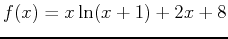 over the interval
 ![$[-1,5]$](img23.png) using right-endpoint and midpoint rules with 6 rectangles.
using right-endpoint and midpoint rules with 6 rectangles.
Next: About this document ...
Up: lab_template
Previous: lab_template
Dina J. Solitro-Rassias
2016-09-05