One of the basic useful principles of analyzing distributed forces is
the idea of replacing them with a single, aggregate force ![]() that acts at a single point and is somehow equivalent to the original
distributed force. This may not always be possible, but this technique
has found great use in engineering and science. As a simple example,
suppose we have gravity acting on a solid plate of uniform thickness and
density, but
irregular shape. Finding the equivalent force is really the problem of
finding the point where we could exactly balance the plate. This
balance point is often called the center of mass of the body.
that acts at a single point and is somehow equivalent to the original
distributed force. This may not always be possible, but this technique
has found great use in engineering and science. As a simple example,
suppose we have gravity acting on a solid plate of uniform thickness and
density, but
irregular shape. Finding the equivalent force is really the problem of
finding the point where we could exactly balance the plate. This
balance point is often called the center of mass of the body.
For symmetric objects, the balance point is usually easy to find. For example, the balance point of an empty see-saw is the exact center. Similarly, the balance points for rectangles or circles are just the geometrical centers. For non-symmetric objects, the answer is not so clear, but it turns out that there is a fairly simple algorithm involving integrals for determining balance points.
We begin by restricting our attention to thin plates of uniform
density. In Engineering and Science, this type of object is called a
lamina. For mathematical purposes, we assume that the lamina is
bounded by ![]() ,
, ![]() ,
, ![]() , and
, and ![]() , with
, with
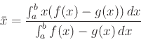
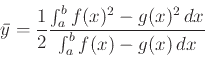
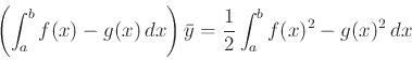
![]() . Then the book gives the following formulas for the coordinates
. Then the book gives the following formulas for the coordinates
![]() of the center of mass.
of the center of mass.
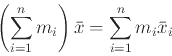
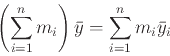
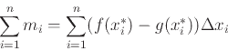
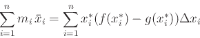
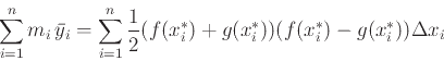
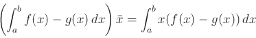
To go from these formulas to the integral formulas presented earlier,
we first partition the interval ![]() into
into ![]() subintervals
subintervals
We end this section with an example, including Maple commands, for
computing the center of mass. Suppose you have a lamina bounded by the
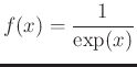
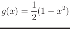
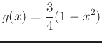
curves
![]() ,
, ![]() , for
, for
![]() and you
want to compute the center of mass, assuming that the density is constant
and you
want to compute the center of mass, assuming that the density is constant ![]() . To do this in Maple, we first
define the two functions.
. To do this in Maple, we first
define the two functions.
> f := x -> x^3-3*x^2-x+3
> g := x -> 3-x
If you are not sure about the relative positions of the two curves, it is a good idea to plot them both.
> plot([g(x),f(x)],x=-2..4)Notice that the graph of
> a := fsolve(f(x)=g(x),x=-1..1)
> b := fsolve(f(x)=g(x),x=1..4)
Now we are ready to compute the center of mass. Using labels, as shown below, can help you organize your calculations and avoid mistakes. Computing the mass separately also lets you check it. If you get a negative value for the mass, something is wrong and you have to check what you have done. A common mistake is reversing the order of the functions.
> mass := int(g(x)-f(x),x=a..b)
> xbar := int(x*(g(x)-f(x)),x=a..b)/mass;
> ybar := 1/2*int(g(x)^2-f(x)^2,x=a..b)/mass;
Finally, you may want to plot the center of mass on the same graph as the functions to see if the center of mass makes sense.
> plot([g(x),f(x),[[xbar,ybar]]],x=a..b,style=[line,line,point],color=black,symbolsize=20)
 and
and
 . Plot both functions on the same graph along with the point
 . Plot both functions on the same graph along with the point