Next: About this document ...
Up: lab_template
Previous: lab_template
Subsections
The purpose of this lab is to give you practice with using integrals
to determine the centroids of thin plates of uniform thickness and
density, but irregular shape.
In designing mechanisms or structures, one often has to deal with
distributed forces, that is, forces that do not act at a discrete,
finite set of points. The most common example of a distributed force
is the force of gravity, which acts on all parts of any body of
matter. Other examples are pressure in fluids and electrostatic
forces, though there are many others.
One of the basic useful principles of analyzing distributed forces is
the idea of replacing them with a single, aggregate force  that acts at a single point and is somehow equivalent to the original
distributed force. This may not always be possible, but this technique
has found great use in engineering and science. As a simple example,
suppose we have gravity acting on a solid plate of uniform thickness and
density, but
irregular shape. Finding the equivalent force is really the problem of
finding the point where we could exactly balance the plate. This
balance point is often called the center of mass of the body.
that acts at a single point and is somehow equivalent to the original
distributed force. This may not always be possible, but this technique
has found great use in engineering and science. As a simple example,
suppose we have gravity acting on a solid plate of uniform thickness and
density, but
irregular shape. Finding the equivalent force is really the problem of
finding the point where we could exactly balance the plate. This
balance point is often called the center of mass of the body.
For symmetric objects, the balance point is usually easy to find. For
example, the balance point of an empty see-saw is the exact center.
Similarly, the balance points for rectangles or circles are just
the geometrical centers. For non-symmetric objects, the answer is not
so clear, but it turns out that there is a fairly simple algorithm
involving integrals for determining balance points.
We begin by restricting our attention to thin plates of uniform
density. In Engineering and Science, this type of object is called a
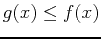
lamina. For mathematical purposes, we assume that the lamina is
bounded by  ,
,  ,
,  , and
, and  , with
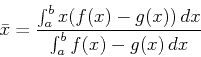
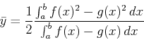
 . Then the book gives the following formulas for the coordinates
 of the center of mass.
We end this section with an example, including Maple commands, for
computing the center of mass. Suppose you have a lamina bounded by the
curves
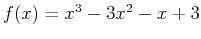 ,
,  and you want to compute the center of mass. To do this in Maple, we first
define the two functions.
and you want to compute the center of mass. To do this in Maple, we first
define the two functions.
> f := x -> x^3-3*x^2-x+3;
> g := x -> 3-x;
Next you need to find the intersection of the two functions. These intersection points will be used as the limits of intgration.
> solve(f(x)=g(x),x);
> plot({g(x),f(x)},x=0..3);
Notice that the graph of  is above the graph of
  . This means
that you must switch and in the formulas.
. This means
that you must switch and in the formulas.
Now we are ready to compute the center of mass. Using labels, as shown
below, can help you organize your calculations and avoid
mistakes. Computing the mass separately also lets you check it. If you
get a negative value for the mass, something is wrong and you have to
check what you have done. A common mistake is reversing the order of
the functions.
> mass := int(g(x)-f(x),x=0..3);
> x_bar := int(x*(g(x)-f(x)),x=0..3)/mass;
> y_bar := 1/2*int(g(x)^2-f(x)^2,x=0..3)/mass;
- Consider the lamina bounded by the curves
 and
and
 .
.
- A)
- Find the intersection points of the two functions.
- B)
- Plot the two functions using the intersection points as the domain.
- C)
- Assume constant density and find the center of mass of the lamina. Does the center of mass lie inside or outside of the lamina?
- Now consider the lamina bounded by the curves
and
 .
.
- A)
- Find the intersection points of the two functions.
- B)
- Plot the two functions using the intersection points as the domain.
- C)
- Assume constant density and find the center of mass of the lamina. Does the center of mass lie inside or outside of the lamina?
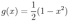
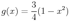
- Finally, consider the lamina bounded by the curves
and
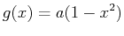 where
where
 .
.
- A)
- Without plotting the lamina, assume constant density and explain why the x coordinate of the center of mass will be
 no matter the value of
  .
.
- B)
- Without plotting the lamina, assume constant density and find the y coordinate of the center of mass in terms of .
- C)
- Again, assume constant density and determine the values of for which the center of mass lies inside the lamina. (Hint: At
 , the bottom edge of the lamina is at
  ). Plot
  and
and  for
to help you answer the question.
for
to help you answer the question.
Next: About this document ...
Up: lab_template
Previous: lab_template
Dina J. Solitro-Rassias
2015-12-06