Subsections

• Purpose
• Background
• Defining vector valued functions simply in Maple
• Getting Started
• Plotting curves of vector defined functions in the plane
• Derivatives and the slope
• The parametric form of a line
• Arc Length, Speed, and Curvature
• Exercises

Vector Functions - Curves in the Plane

Purpose

The purpose of this lab is to introduce you to curve computations using Maple for parametric curves and vector-valued functions in the plane.

Background

Defining vector valued functions simply in Maple

The easiest way to define a vector function or a parametric curve is to use the Maple list notaion with square brackets[]. Strictly speaking, this does not define something that Maple recognizes as a vector, but it will work with all of the commands you need for this lab.

Getting Started

To assist you, there is a worksheet associated with this lab that contains examples similar to some of the exercises.On your Maple screen go to File - Open then type the following in the white rectangle:

\\storage\academics\math\calclab\MA1023\Vector_start_A14.mw

You can copy the worksheet now, but you should read through the lab before you load it into Maple. Once you have read through the exercises, start up Maple, load the worksheet, and go through it carefully. Then you can start working on the exercises.

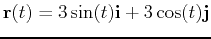
>r:=t->[3*sin(t),3*cos(t)];

You can evaluate this function at any value of t in the usual way.

>r(0);

This is how to access a single component.

>r(t)[1];
>r(t)[2];

Plotting curves of vector defined functions in the plane

The VPlot command is in the CalcP package so you have to load it first. If you get an error from this command, ask for help right away. A few examples are shown below.

>with(CalcP7):
>VPlot([t^2,t^3-t],t=-1.5..1.5);
>VPlot(r(t),t=0..2*Pi);

Derivatives and the slope

The graph of a parametric curve may not have a slope at every point on the curve. When the slope exists, it is given by the formula:

$$\frac{dy}{dx} = \frac{\frac{dy}{dt}}{\frac{dx}{dt}}$$

In Maple, the slope of a parametric curve can be calculated using the $\texttt{diff}$ command as in the example below.

> r := -> [3*sin(t),3*cos(t)];
> slope := diff(r(t)[2],t)/diff(r(t)[1],t);

The parametric form of a line

The vector equation for the line passing through the point $\mathbf{r_0}=(x_0,y_0)$ parallel to the vector $\mathbf{v}=[v_1,v_2]$ is given by:

$$\mathbf{r}(t) = \mathbf{r}_0 + t\mathbf{v}$$

Below is an example in Maple using this parametric form of a line that is tangent to the curve $\mathbf{r}(t)$ defined above at $$t=\frac{\pi}{4}$$. The plot of the curve and the line on the same graph verifies that the line is tangent at the given point.

>eval(slope,t=Pi/4);

Since the slope at $$\frac{\pi}{4}$$ is -1, we want the line through the point $$\mathbf{r}(\frac{\pi}{4})$$, parallel to the vector $[1,-1]$.

>line:=t->r(Pi/4)+[t,-t];
>with(plots):
>a:=VPlot(r(t),t=-Pi..Pi):
>b:=VPlot(line(t),t=-Pi..Pi):
>display(a,b);

Arc Length, Speed, and Curvature

Parametric curves often represent the motion of a particle or mechanical system. When we think of a parametric curve as representing motion, we need a way to measure the distance traveled by the particle. This distance is given by the arc length, $s$, of a curve. For a parametric curve $\mathbf{r}(t) = f(t) \mathbf{i} + g(t) \mathbf{j}$, the arc length of the curve for $a \leq t \leq b$ is given below.

$$s = \int_{a}^{b} \sqrt{ (f'(t))^2+(g'(t))^2} \, dt$$

While the concept of arc length is very useful for the theory of parametric curves, it turns out to be very difficult to compute in all but the simplest cases. The maple command below shows that the arclength of a circle with the parametrization $\mathbf{r}(t) = 3\sin(t) \mathbf{i} + 3\cos(t) \mathbf{j}$ has constant arclength.

> evalf(int(sqrt(diff(3*sin(t),t)^2+diff(3*cos(t),t)^2),t=0..2*Pi));

For this lab, we will also assume that we have a vector-valued function ${\bf r}(t)$ that gives the position at time $t$ of a moving point $P$ in the plane. The velocity of this point is given by the derivative ${\bf r}'(t)$ and the acceleration is given by the second derivative, ${\bf r}''(t)$. In many applications of curvilinear motion, we need to know the magnitude of the velocity, or the speed. This is easy to compute - just take the magnitude $\vert{\bf r}'(t)\vert$. If you think of the speed as the rate of change of distance along the curve, and recall that arc length is distance measured along the curve, then you have the following interpretation of the speed

$$\frac{ds}{dt} = \vert{\bf r}'(t)\vert$$

where $S$ is arc length. If the speed is not zero for any value of $t$ in the interval $I$, then it is possible to define a unit vector, ${\bf T}(t)$ that is tangent to the curve as follows.

$${\bf T}(t)= \frac{{\bf r}'(t)}{\vert{\bf r}'(t)\vert}$$

Using this definition, you can write the velocity in the following form.

$${\bf r}'(t) = \frac{ds}{dt} {\bf T}(t)$$

This is not the most useful form for calculating the velocity, but it does lead to a useful way of thinking about the acceleration experience by a particle moving in a curvilinear path. If the path is a straight line, acceleration depends only on whether the particle is speeding up or slowing down. In a curve, however, there is an additional acceleration, called the centripetal acceleration, that is needed to keep the particle moving on the curve. The magnitude of this acceleration depends on the speed of the car and how much the path is curving. It turns out that you can quantify this with an intrinsic property of the curve called the curvature, usually denoted $\kappa$, defined by the following equation.

$$\kappa = \vert\frac{d{\bf T}}{ds}\vert = \frac{1}{\vert\bf v\vert} \vert\frac{d \bf T}{dt}\vert$$

That is, the curvature is the magnitude of the rate of change of the tangent vector $T$ with respect to arc length. For example, the curvature of a straight line is zero and it can be shown that the curvature of a circle of radius $R$ is the same for every point on the circle and is given by $\kappa = 1/R$. The Maple Speed command computes the speed of a vector function and the Curvature command computes the curvature of a vector function. The syntax for these commands is shown in the example below that computes the speed of a particle traveling along the path traced by the curve $\mathbf{r}(t)=3\cos(t)\mathbf{i} + 3\sin(t)\mathbf{j}$at $t=\pi$, the curvature of the curve at $t=\pi$ and the arclength of the curve over the interval $0 \leq t \leq 2\pi$.

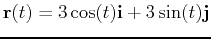
> r:=t->[3cos(t),3sin(t)];
> v:=diff(r(t),t);
> sqrt(v[1]^2+v[2]^2);
> Speed(r(t),t);
> Speed(r(t),t=Pi);
> Curvature(r(t),t=Pi);
> int(sqrt(v[1]^2+v[2]^2),t=0..2*Pi);

Exercises

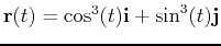
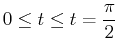
1. Consider the vector function $\mathbf{r}(t) = (2\cos(t) + 4\cos^2(t))\mathbf{i} + (2\sin(t) + 4\sin(t)\cos(t))\mathbf{j}$ for $-\pi \leq t \leq \pi$.
   1. Calculate the $(x,y)$ coordinate point on the curve at $$t =-\frac{\pi}{2}$$ and the slope of the curve at $$t =-\frac{\pi}{2}$$.
   2. Define the vector equation of the line through the point above tangent to the curve at that point.
   3. Plot the graph of $\mathbf{r}(t)$ and this tangent line on the same graphover the interval $-\pi \leq t \leq \pi$.
2. Given the vector function $\mathbf{r}(t) = \cos^3(t)\mathbf{i} + \sin^3(t)\mathbf{j}$
   1. Plot the vector function over the interval $$0 \leq t \leq t=\frac{\pi}{2}$$.
   2. Calculate the speed of the particle at $$t=\frac{\pi}{4}$$ using the magnitude of the velocity and verify using Maple's Speed command. Calculate the curvature at $$t=\frac{\pi}{4}$$ using Maple's Curvature command.
   3. Calculate the arclength $\mathbf{r}(t)$ over the interval $0 \leq t \leq \frac{\pi}{2}$.