


Next: About this document ...
Up: lab_template
Previous: lab_template
Subsections
The use of parametric equations and polar coordinates allows for the analysis of families of curves difficult to handle through rectangular coordinates. If a curve is a rectangular coordinate graph of a function, it cannot have any loops since, for a given  value there can be at most one corresponding
  value. However, using polar coordinates, curves with loops can appear as graphs of functions.
To assist you, there is a worksheet associated with this lab that
contains examples similar to some of the exercises. You can access this worksheet by typing in the search field (magnifying glass next to start menu):
\\storage.wpi.edu\academics\math\calclab\MA1023\Parametric_polar_start_A19.mw
A parametric curve in the plane is represented by a pair of equations  and
and  for t in some interval I. A vector-valued function in
the plane is a function
for t in some interval I. A vector-valued function in
the plane is a function  that associates a vector in
the plane with each value of
that associates a vector in
the plane with each value of  in its domain. Such a vector valued function can always be written in component form as follows,
where  and
and  are functions defined on some interval
  . From our
definition of a parametric curve, it should be clear that you can
always associate a
parametric curve with a vector-valued function by just considering the
curve traced out by the head of the vector.
. From our
definition of a parametric curve, it should be clear that you can
always associate a
parametric curve with a vector-valued function by just considering the
curve traced out by the head of the vector.
The ParamPlot command is in the CalcP package so you have to load it first. If you get an error from this command, ask for help right away.
>with(CalcP7):
The ParamPlot command produces an animated plot. To see the animation, execute the command and then click on the plot region below to make the controls appear in the Context Bar just above the worksheet window. When the controls appear, you can click on the play button to animate the curve.
For a curve defined parametrically by the equations and ,
> f:=t->cos(t)
> g:=t->sin(t)
The parametric curve can be plotted with or without animation:
> with(CalcP7):
> plot([f(t),g(t),t=0..2Pi])
> ParamPlot([f(t),g(t)],t=0..2Pi)
Both plots show that the given parametric curve is a circle. The plot command only shows the final curve whereas the ParamPlot command shows starting point, ending point and direction of motion.
When you graph curves in polar coordinates, you are really working with parametric curves. The basic idea is that you want to plot a set of points by giving their coordinates in  pairs. When you use polar coordinates, you are defining the points in terms of polar coordinates
  where
where
 and
and
 . When you plot polar curves, you are usually assuming that
  is a function of the angle
  and is the parameter that describes the curve.
In Maple you have to put square brackets around the curve and add the specification coords=polar. Maple assumes that the first coordinate in the parametric plot is the radius
and is the parameter that describes the curve.
In Maple you have to put square brackets around the curve and add the specification coords=polar. Maple assumes that the first coordinate in the parametric plot is the radius  and the second coordinates is the angle
  .
.
Other than circles, there are three types of well-known graphs in polar coordinates. The
table below will allow you to identify the graphs in the exercises.
| Name |
Equation |
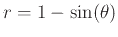
| cardioid |
 or or
 |
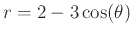
| limaçon |
 or or
 |
| rose |
 or or
 |
Below is an example of how to plot and animate the circle
 using a polar plot in Maple.
> plot(cos(theta),theta=0..2Pi,coords=polar)
> plots[animate](plot,[cos(theta),theta=0..t,coords=polar],t=0..2Pi)
- Consider the simple function
 . Animate the following two parameterizations
 for this curve for
 and state how the two parameterizations of the same function are different.
- Find two different parametrizations of a semi-circle of radius 2, centered at the origin, one with and one without using trig functions for
 and
and  , the necessary interval of t for each, and plot each of the parametric curves on separate graphs using ParamPlot.
- Plot each of the polar graphs below and identify the name of the polar graph using the table in the background.
- a)
-

- b)
-
- c)
-
- a)
- Animate the plot of the three-petal rose
 in polar coordinates over the interval
 and again over the interval
 . What is the necessary interval of values needed to traverse the polar plot exactly once? Find the angles that create only one petal of the rose
. Plot exactly one petal.
. What is the necessary interval of values needed to traverse the polar plot exactly once? Find the angles that create only one petal of the rose
. Plot exactly one petal.
- b)
- Repeat part a with
 .
.
Next: About this document ...
Up: lab_template
Previous: lab_template
Dina J. Solitro-Rassias
2019-09-12