Next: About this document ...
Up: lab_template
Previous: lab_template
Subsections
The purpose of this lab is to use Maple to introduce you to
Taylor polynomial approximations to functions, including some
applications.
To assist you, there is a worksheet associated with this lab that
contains examples similar to some of the exercises. You can access this worksheet by typing in the search field (magnifying glass next to start menu):
\\storage.wpi.edu\academics\math\calclab\MA1023\Taylor_start_A19.mw
The idea of the Taylor polynomial approximation of order  at
at
 , written
  , to a smooth function
  is to require
that and have the same value at .
Furthermore, their derivatives at must match up to order
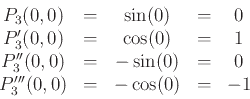
. For example the Taylor polynomial of order three for
is to require
that and have the same value at .
Furthermore, their derivatives at must match up to order
. For example the Taylor polynomial of order three for  at
at
 would have to satisfy the conditions
You should check for yourself that the cubic polynomial satisfying
these four conditions is
The general form of the Taylor polynomial approximation of order
to is given by the following
Theorem 1
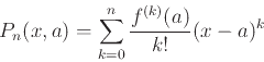
Suppose that is a smooth function in some open interval
containing . Then the th degree Taylor polynomial of the
function at the point is given by
The notation
 is used in the definition to stand for the value of the
 -th derivative of
  at . That is,
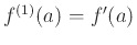 ,
,
 , and so on. By convention,
 . Note that
  is fixed and so the derivatives are
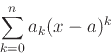
just numbers. That is, a Taylor polynomial has the form
is fixed and so the derivatives are
just numbers. That is, a Taylor polynomial has the form
which you should recognize as a power series that has been truncated.
To measure how well a Taylor Polynomial approximates the function over
a specified interval ![$[c,d]$](img19.png) , we define the tolerance
, we define the tolerance  of
to be the maximum of the absolute error
of
to be the maximum of the absolute error
over the interval .
To use the Taylor and TayPlot commands you need to load the CalcP7 package.
> with(CalcP7):
We know that a linear approximation to a function at a point is the tangent line at that point. You can see that the first order Taylor polynomial is the tangent line. A second degree polynomial would be a better approximation as it not only has the same slope as the function, but the same concavity at the base point.
The example below shows the exponential function  approximated at a base point zero with a polynomial of order 1 and order 2 and plotted on the same graph as using the following commands:
> f:=x->exp(x)
> tp1 := Taylor(f(x),x=0,1)
> plot([f(x),tp1],x=-2..2)
> tp2 := Taylor(f(x),x=0,2)
> plot([f(x),tp2],x=-2..2)
The approximation is better as you increase the order of the Taylor polynomial. To see this effect, you might want to experiment with changing the order and observe the change in absolute error. Suppose you want to use the Taylor polynomial for
with base point to approximate  with error no greater than 0.1. The commands below show how you can check the absolute error as you increase the order of the Taylor polynomial.
> tp := Taylor(f(x),x=0,1)
> evalf(abs(f(1)-subs(x=1,tp)))
> tp := Taylor(f(x),x=0,2)
> evalf(abs(f(1)-subs(x=1,tp)))
> tp := Taylor(f(x),x=0,5)
> evalf(abs(f(1)-subs(x=1,tp)))
The command below allows you to see the exponential function and three approximating polynomials on the same graph.
> TayPlot(f(x),x=0,{1,2,3},x=-2..2)
Notice that the further away from the base point, the further the polynomial diverges from the function. the amount the polynomial diverges i.e. its error, is simply the difference of the function and the polynomial. To see how well the Taylor polynomial approximates a function over an interval, we can plot the error.
> plot([abs(f(x)-Taylor(f(x),x=0,3)),0.1],x=-2..2,y=0..0.15)
This plot shows that in the domain x from -2 to 2 the error around the base point is zero and the error is its greatest at x = 2 with a difference of over one. You can experiment with the polynomial orders to change the accuracy. If your work requires an error of no more than 0.2 within a given distance of the base point then you can plot your accuracy line y = 0.1 along with the difference of the function and the Taylor approximation polynomial.
We knew this would have some of its error well above 0.2. Change the order from three to four. As you can see there are still some values in the domain close to x = 2 whose error is above 0.2. Now try an order of 5. Is the error entirely under 0.2 between x = -2 and x = 2? Larger orders will work as well but order five is the minimum order that will keep the error under 0.2 within the given domain.
- For the function
 ,
,
- a)
- Find the first order Taylor polynomial for about the base point and plot it on the same graph as over the interval
![$[-2,2]$](img25.png) . Then, determine the absolute error when approximating using this first order Taylor polynomial.
. Then, determine the absolute error when approximating using this first order Taylor polynomial.
- b)
- Find the second order Taylor polynomial for about the base point and plot it on the same graph as over the interval . Then, determine the absolute error when approximating using this second order Taylor polynomial.
- c)
- Find the minimum order Taylor polynomial for , with base point , needed to approximate with absolute error no greater than 0.1.
- d)
- Find the minimum order Taylor polynomial for , with base point , needed to approximate
 with absolute error no greater than 0.1.
- e)
- Find the minimum order Taylor polynomial for , with base point , needed to approximate
 with absolute error no greater than 0.1.
- For the function,
 , use the TayPlot command to plot the function and multiple Taylor polynomial approximations of various orders with base point on the same graph over the interval
 ; also use a y-range
 .
.
- a)
- If you increase the order of the Taylor polynomial, can you get a good approximation at
 ?
?
- b)
- Can you make a guess for the interval or radius of convergence. That is, an interval of
 values for which the Taylor polynomial converges to the function and outside that interval, does not converge to the function. Explain how this interval can be verified based on what you know about convergence of geometric series.
Next: About this document ...
Up: lab_template
Previous: lab_template
Dina J. Solitro-Rassias
2019-09-23