


Next: About this document ...
Up: lab_template
Previous: lab_template
Subsections
The purpose of this lab is to give you some experience with using the
trapezoidal rule and Simpson's rule to approximate integrals.
To assist you, there is a worksheet associated with this lab that
contains examples and even solutions to some of the exercises. You can
copy that worksheet to your home directory with the following command,
which must be run in a terminal window, not in Maple.
cp /math/calclab/MA1023/NumInt_start.mws ~
You can copy the worksheet now, but you should read through the lab
before you load it into Maple. Once you have read to the exercises,
start up Maple, load
the worksheet NumInt_start.mws, and go through it
carefully. Then you can start working on the exercises.
In class we have talked about the trapezoidal rule and Simpson's rule
for approximating the definite integral
Both methods start by dividing the interval ![$[a,b]$](img2.png) into
into  subintervals of equal length by choosing a partition
satisfying
where
is the length of each subinterval. For the trapezoidal rule, the
integral over each subinterval is approximated by the area of a
trapezoid. This gives the
following approximation to the integral
For Simpson's rule, the function is approximated by a parabola over
pairs of subintervals. When the areas under the parabolas are computed
and summed up, the result is the following approximation.
There are many times in math, science, and engineering that coordinate
systems other than the familiar one of Cartesian coordinates are
convenient. In this lab, we consider one of the most common and useful
such systems, that of polar coordinates.
The main reason for using polar coordinates is that they can be used
to simply describe regions in the plane that would be very difficult
to describe using Cartesian coordinates. For example, graphing the
circle  in Cartesian coordinates requires two functions -
one for the upper half and one for the lower half. In polar
coordinates, the same circle has the very simple representation
in Cartesian coordinates requires two functions -
one for the upper half and one for the lower half. In polar
coordinates, the same circle has the very simple representation  .
.
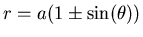
These are three types of well-known graphs in polar coordinates. The
table below will allow you to identify the graphs in the exercises.
| Name |
Equation |
| cardioid |
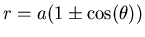 or or
 |
| limaçon |
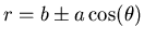 or or
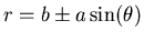 |
| rose |
 or or
 |
Finding where two graphs in Cartesian coordinates intersect is
straightforward. You just set the two functions equal and solve for
the values of  . In polar coordinates, the situation is more
difficult. Most of the difficulties are due to the following considerations.
. In polar coordinates, the situation is more
difficult. Most of the difficulties are due to the following considerations.
- A point in the plane can have more than one representation in
polar coordinates. For example, ,
 is the same
point as
is the same
point as  ,
,  . In general a point in the plane can have
an infinite number of representations in polar coordinates, just by
adding multiples of
. In general a point in the plane can have
an infinite number of representations in polar coordinates, just by
adding multiples of  to
to  . Even if you restrict
a point in the plane can have several different representations.
. Even if you restrict
a point in the plane can have several different representations.
- The origin is determined by
 . The angle can have
any value.
. The angle can have
any value.
These considerations can make finding the intersections of two graphs in polar
coordinates a difficult task. As the exercises demonstrate, it
usually requires a combination of plots and solving equations to find
all of the intersections.
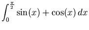
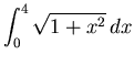
- For each of the definite integrals given below, find the exact value of the integral using the int command. Then find the minimum number of subintervals needed to approximate the integral using the trapezoidal rule and then again using Simpson's rule with and error no greater than 0.001. Which method is better and why?
-
-
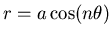
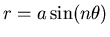
- Find all points of intersection for the pair of curves in polar
coordinates given by the equations
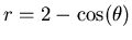 and
and
 for
for
 .
.
Next: About this document ...
Up: lab_template
Previous: lab_template
Dina Solitro
2004-11-22