Subsections

• Purpose
• Background
• Plotting and animating curves in the plane
• Defining parametric curves and vector valued functions simply in Maple
  • Derivatives and the slope
  
  
• The parametric form of a line
  • Arc length
  
  
• Exercises

Parametric Curves in the Plane

Purpose

The purpose of this lab is to introduce you to curve computations using Maple for parametric curves and vector-valued functions in the plane.

Background

By parametric curve in the plane, we mean a pair of equations $x=f(t)$ and $y=g(t)$ for $t$ in some interval $I$. A vector-valued function in the plane is a function $\mathbf{r}(t)$ that associates a vector in the plane with each value of $t$ in its domain. Such a vector valued function can always be written in component form as follows,

$$\mathbf{r}(t) = f(t) \mathbf{i} + g(t) \mathbf{j}$$

where $f$ and $g$ are functions defined on some interval $I$. From our definition of a parametric curve, it should be clear that you can always associate a parametric curve with a vector-valued function by just considering the curve traced out by the head of the vector.

Plotting and animating curves in the plane

The ParamPlot command is in the CalcP package so you have to load it first. If you get an error from this command, ask for help right away.

>with(CalcP7);

The ParamPlot command produces an animated plot. To see the animation, execute the command and then click on the plot region below to make the controls appear in the Context Bar just above the worksheet window.

>ParamPlot([t,t^2],t=-2..2);

the direction of the motion on the curve can be reversed by simply changing the first component from t to -t, as shown below.

>ParamPlot([-t,t^2],t=-2..2);

The ParamPlot command is nice for visualization, but its output doesn't always show up in printouts. Toproduce a printable plot, you can use the VPlot command as shown below.

>VPlot([t^2,t^3-t],t=-1.5..1.5);

Defining parametric curves and vector valued functions simply in Maple

The easiest way to define a vector function or a parametric curve is to use the Maple list notaion with square brackets[]. Strictly speaking, this does not define something that Maple recognizes as a vector, but it will work with all of the commands you need for this lab.

>f:=t->[2*cos(t),2*sin(t)];

You can evaluate this function at any value of t in the usual way.

>f(0);

This is how to access a single component. You would use f(t)[2] to get the second component.

>f(t)[1]

Derivatives and the slope

The graph of a parametric curve may not have a slope at every point on the curve. When the slope exists, it must be given by the formula from class.

$$\frac{dy}{dx} = \frac{\frac{dy}{dt}}{\frac{dx}{dt}}$$

It is clear that this formula doesn't make sense if $$\frac{dx}{dt}= 0$$ at some particular value of $t$. If $$\frac{dy}{dt} \neq 0$$ at that same value of $t$, then it turns out the graph has a vertical tangent at that point. If both $$\frac{dx}{dt}$$ and $$\frac{dy}{dt}$$ are zero at some value of $t$, then the curve often doesn't have a tangent line at that point. What you see instead is a sharp corner, called a cusp. An example of this appears in the first exercise.

The parametric form of a line

The vector equation for the line passing through the point $\mathbf{r_0}=(x_0,y\ _0)$ parallel to the vector $\mathbf{v}=[v_1,v_2]$ is given by:

$$\mathbf{r}(t) = \mathbf{r}_0 + t\mathbf{v}$$

Below is an example in Maple using this parametric form of a line that is tange nt to the curve $\mathbf{r}(t)$ defined above at $$t=\frac{\pi}{4}\$$. The plot of the curve and the line on the same graph verifies that the line is tangent at the given point.

>eval(slope,t=Pi/4);

Since the slope at $$\frac{\pi}{4}$$ is -1, we want the line throug h the point $$\mathbf{r}(\frac{\pi}{4})$$, parallel to the vector $\ [1,-1]$.

>line:=t->r(Pi/4)+[t,-t];
>with(plots):
>a:=VPlot(r(t),t=-Pi..Pi):
>b:=VPlot(line(t),t=-Pi..Pi):
>display(a,b);

Arc length

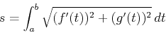
As mentioned above, parametric curves often represent the motion of a particle or mechanical system. As we will see in class, when we think of a parametric curve as representing motion, we need a way to measure the distance traveled by the particle. This distance is given by the arc length, $s$, of a curve.

For a parametric curve $x=f(t)$, $y=g(t)$, the arc length of the curve for $a \leq t \leq b$ is given below.

$$s = \int_{a}^{b} \sqrt{ (f'(t))^2+(g'(t))^2} dt$$

While the concept of arc length is very useful for the theory of parametric curves, it turns out to be very difficult to compute in all but the simplest cases.

Exercises

1. Plot the curve
   
   $$\mathbf{r}(t) = (5\cos(t)+\cos(5t)) \mathbf{i} + (5\sin(t)-\sin(5t)) \mathbf{j}$$
   
   
   for $0 \leq t \leq 2\pi$.
   1. Find the formula for the slope of the parametric curve.
   2. Find $t$ values for two points on the graph where the slope does not exist or where there is a cusp.
   3. Calculate the $(x,y)$ coordinate location for the two points above and plot them on the graph along with the parametrization. You will find some of the commands below helpful, but you will need more commands than what is given.

      >xp:=diff(r(t)[1],t);
      >solve({xp=0,yp=0},t);
      >r(0);
      >with(plots):
      >a:=VPlot(r(t),t=0..2*Pi):
      >b:=VPlot(r(0),t=0..2*Pi,style=point,symbolsize=30,color=black):
      >display(a,b,c);
      

2. Consider the vector function $\mathbf{r}(t) = (2\cos(t) + 4\cos^2(t))\mathbf{i} + (2\sin(t) + 4\sin(t)\cos(t))\mathbf{j}$ for $-\pi \leq t \leq \pi$.
   1. Calculate the $(x,y)$ coordinate point on the curve at $$t =\ -\frac{\pi}{2}$$ and the slope of the curve at $$t = -\frac{\pi}{2}\$$.
   2. Define the vector equation of the line through the point above tangent to the curve at that point.
   3. Plot the graph of $\mathbf{r}(t)$ and this tangent line on the same graph over the interval $-\pi \leq t \leq \pi$.

3. For the ellipse
   
   $$\frac{x^2}{16}+ \frac{y^2}{36} = 1$$
   
   
   , plot the ellipse implicityly and calculate the arclength directly using the commands given below:

   > with(plots):
   > implicitplot(x^2/16+y^2/36=1,x=-4..4,y=-6..6,scaling=constrained)
   > f := solve(x^2/16+y^2/36=1, y)
   > df := diff(f[1],x)
   > evalf(2*int(sqrt(1+df^2),x=-4..4))
   

   Next, define the ellipse parametrically, $x(t)$ and $y(t)$, and determine the necessary interval for the ellipse. Use VPlot to show that they are the same ellipse (you may want to use scaling=constrained) and find the arclength of the ellipse using the parametrizations.